W4:multi-class classification

Week4 Multiclass Classifications

You’ve come a long way, Congratulations! One more thing to do before we move off of ConvNets to the next module, and that’s to go beyond binary classification. Each of the examples you’ve done so far involved classifying one thing or another – horse or human, cat or dog. When moving beyond binary into Categorical classification there are some coding considerations you need to take into account. You’ll look at them this week!

Code

import os
import zipfile
import random
import shutil
import tensorflow as tf
from tensorflow.keras.optimizers import RMSprop
from tensorflow.keras.preprocessing.image import ImageDataGenerator
from shutil import copyfile
from os import getcwd

1 download data

download trainning data

Code

import urllib.request
urllib.request.urlretrieve( "https://storage.googleapis.com/learning-datasets/rps.zip", "./tmp/rps.zip")

download testing data

Code

import urllib.request
urllib.request.urlretrieve( "https://storage.googleapis.com/learning-datasets/rps-test-set.zip", "./tmp/rps-test-set.zip")

unzip

Code

import os
import zipfile

local_zip = './tmp/rps.zip'
zip_ref = zipfile.ZipFile(local_zip, 'r')
zip_ref.extractall('./tmp/')
zip_ref.close()

local_zip = './tmp/rps-test-set.zip'
zip_ref = zipfile.ZipFile(local_zip, 'r')
zip_ref.extractall('./tmp/')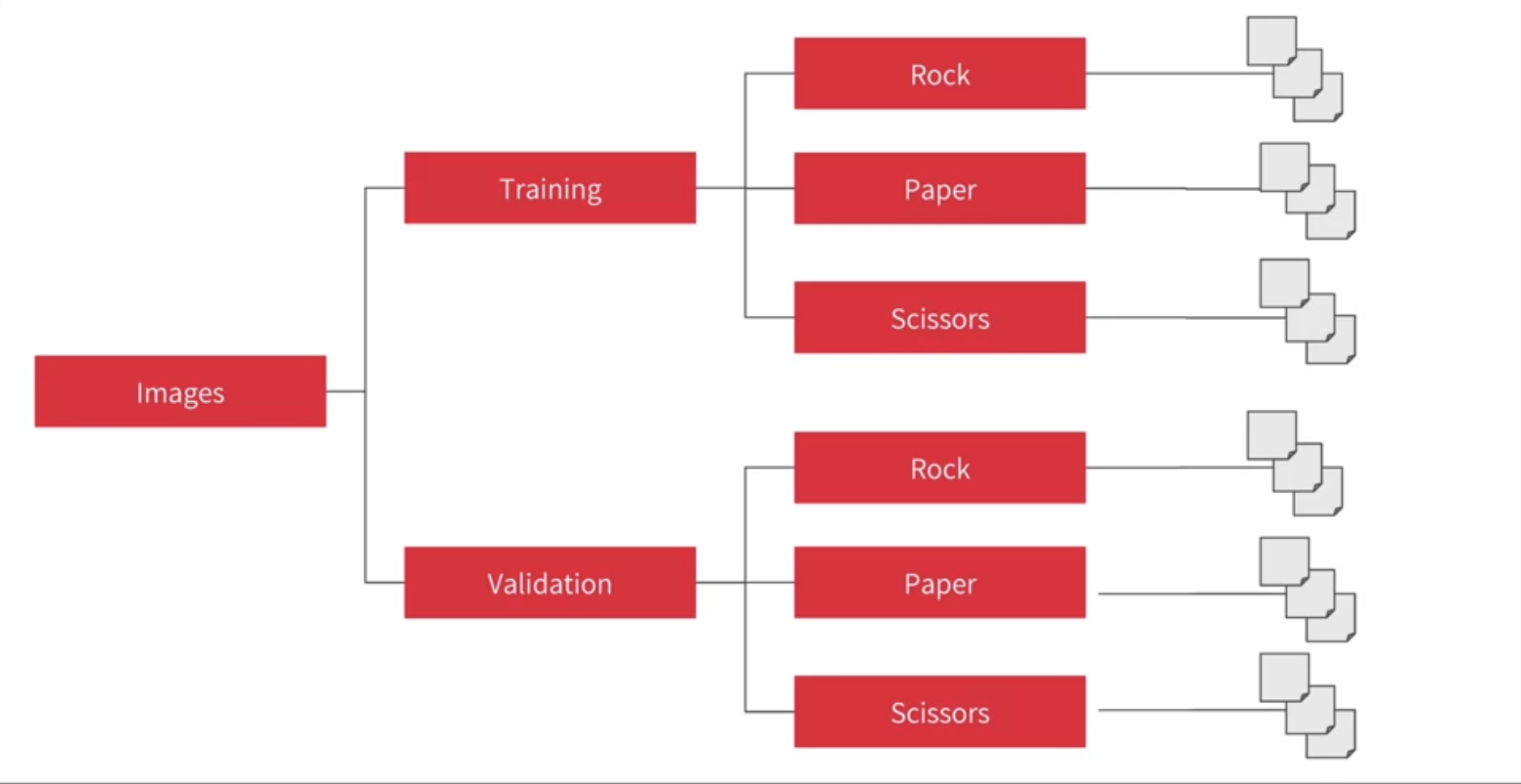
zip_ref.close()

Code

rock_dir = os.path.join('./tmp/rps/rock')
paper_dir = os.path.join('./tmp/rps/paper')
scissors_dir = os.path.join('./tmp/rps/scissors')

print('total training rock images:', len(os.listdir(rock_dir)))
print('total training paper images:', len(os.listdir(paper_dir)))
print('total training scissors images:', len(os.listdir(scissors_dir)))

total training rock images: 840
total training paper images: 840
total training scissors images: 840

Code

rock_files = os.listdir(rock_dir)
print(rock_files[:10])

paper_files = os.listdir(paper_dir)
print(paper_files[:5])

scissors_files = os.listdir(scissors_dir)
print(scissors_files[:5])

['rock04-059.png', 'rock01-108.png', 'rock04-065.png', 'rock05ck01-067.png', 'rock05ck01-073.png', 'rock04-071.png', 'rock05ck01-098.png', 'rock02-008.png', 'rock07-k03-013.png', 'rock02-034.png']
['paper03-088.png', 'paper05-026.png', 'paper05-032.png', 'paper03-077.png', 'paper03-063.png']
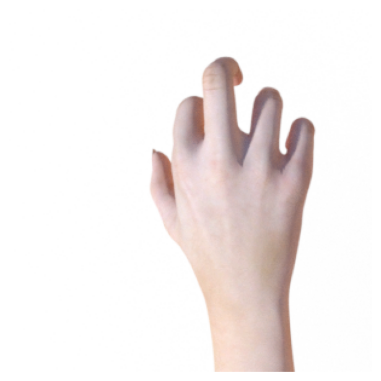
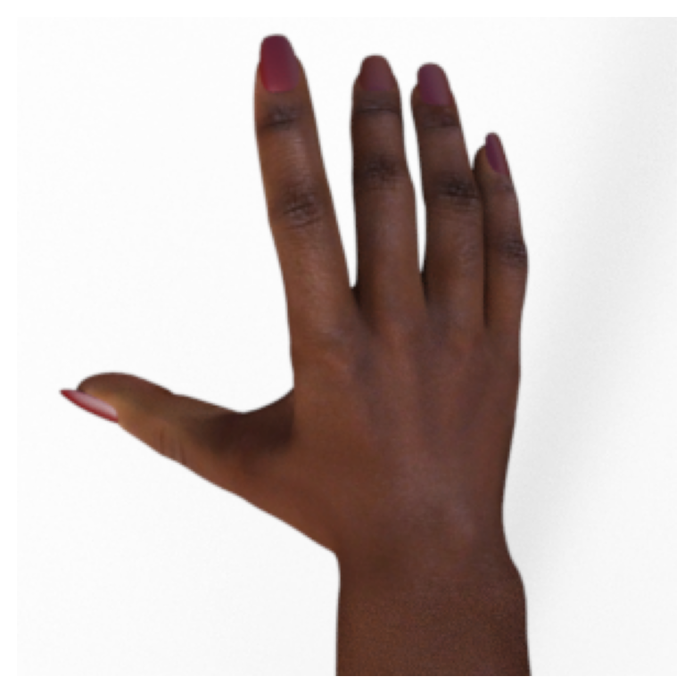
['testscissors03-040.png', 'testscissors03-054.png', 'testscissors03-068.png', 'testscissors03-083.png', 'testscissors03-097.png']

Code

import matplotlib.pyplot as plt
import matplotlib.image as mpimg

pic_index = 2

next_rock = [os.path.join(rock_dir, fname) 
                for fname in rock_files[pic_index-2:pic_index]]
next_paper = [os.path.join(paper_dir, fname) 
                for fname in paper_files[pic_index-2:pic_index]]
next_scissors = [os.path.join(scissors_dir, fname) 
                for fname in scissors_files[pic_index-2:pic_index]]

for i, img_path in enumerate(next_rock+next_paper+next_scissors):
  #print(img_path)
  img = mpimg.imread(img_path)
  plt.imshow(img)
  plt.axis('Off')
  plt.show()

2 load data

Code

import tensorflow as tf
import keras_preprocessing
from keras_preprocessing import image
from keras_preprocessing.image import ImageDataGenerator

TRAINING_DIR = "./tmp/rps/"
training_datagen = ImageDataGenerator(
      rescale = 1./255,
        rotation_range=40,
      width_shift_range=0.2,
      height_shift_range=0.2,
      shear_range=0.2,
      zoom_range=0.2,
      horizontal_flip=True,
      fill_mode='nearest')

Code

VALIDATION_DIR = "./tmp/rps-test-set/"
validation_datagen = ImageDataGenerator(rescale = 1./255)

train_generator = training_datagen.flow_from_directory(
    TRAINING_DIR,
    target_size=(150,150),
    class_mode='categorical',
  batch_size=126
)

validation_generator = validation_datagen.flow_from_directory(
    VALIDATION_DIR,
    target_size=(150,150),
    class_mode='categorical',
  batch_size=126
)

Found 2520 images belonging to 3 classes.
Found 372 images belonging to 3 classes.

3 define model

Code

model = tf.keras.models.Sequential([
    # Note the input shape is the desired size of the image 150x150 with 3 bytes color
    # This is the first convolution
    tf.keras.layers.Conv2D(64, (3,3), activation='relu', input_shape=(150, 150, 3)),
    tf.keras.layers.MaxPooling2D(2, 2),
    # The second convolution
    tf.keras.layers.Conv2D(64, (3,3), activation='relu'),
    tf.keras.layers.MaxPooling2D(2,2),
    # The third convolution
    tf.keras.layers.Conv2D(128, (3,3), activation='relu'),
    tf.keras.layers.MaxPooling2D(2,2),
    # The fourth convolution
    tf.keras.layers.Conv2D(128, (3,3), activation='relu'),
    tf.keras.layers.MaxPooling2D(2,2),
    # Flatten the results to feed into a DNN
    tf.keras.layers.Flatten(),
    tf.keras.layers.Dropout(0.5),
    # 512 neuron hidden layer
    tf.keras.layers.Dense(512, activation='relu'),
    tf.keras.layers.Dense(3, activation='softmax')
])

Code

model.summary()

Model: "sequential"

┏━━━━━━━━━━━━━━━━━━━━━━━━━━━━━━━━━┳━━━━━━━━━━━━━━━━━━━━━━━━┳━━━━━━━━━━━━━━━┓
┃ Layer (type)                    ┃ Output Shape           ┃       Param # ┃
┡━━━━━━━━━━━━━━━━━━━━━━━━━━━━━━━━━╇━━━━━━━━━━━━━━━━━━━━━━━━╇━━━━━━━━━━━━━━━┩
│ conv2d (Conv2D)                 │ (None, 148, 148, 64)   │         1,792 │
├─────────────────────────────────┼────────────────────────┼───────────────┤
│ max_pooling2d (MaxPooling2D)    │ (None, 74, 74, 64)     │             0 │
├─────────────────────────────────┼────────────────────────┼───────────────┤
│ conv2d_1 (Conv2D)               │ (None, 72, 72, 64)     │        36,928 │
├─────────────────────────────────┼────────────────────────┼───────────────┤
│ max_pooling2d_1 (MaxPooling2D)  │ (None, 36, 36, 64)     │             0 │
├─────────────────────────────────┼────────────────────────┼───────────────┤
│ conv2d_2 (Conv2D)               │ (None, 34, 34, 128)    │        73,856 │
├─────────────────────────────────┼────────────────────────┼───────────────┤
│ max_pooling2d_2 (MaxPooling2D)  │ (None, 17, 17, 128)    │             0 │
├─────────────────────────────────┼────────────────────────┼───────────────┤
│ conv2d_3 (Conv2D)               │ (None, 15, 15, 128)    │       147,584 │
├─────────────────────────────────┼────────────────────────┼───────────────┤
│ max_pooling2d_3 (MaxPooling2D)  │ (None, 7, 7, 128)      │             0 │
├─────────────────────────────────┼────────────────────────┼───────────────┤
│ flatten (Flatten)               │ (None, 6272)           │             0 │
├─────────────────────────────────┼────────────────────────┼───────────────┤
│ dropout (Dropout)               │ (None, 6272)           │             0 │
├─────────────────────────────────┼────────────────────────┼───────────────┤
│ dense (Dense)                   │ (None, 512)            │     3,211,776 │
├─────────────────────────────────┼────────────────────────┼───────────────┤
│ dense_1 (Dense)                 │ (None, 3)              │         1,539 │
└─────────────────────────────────┴────────────────────────┴───────────────┘

 Total params: 3,473,475 (13.25 MB)

 Trainable params: 3,473,475 (13.25 MB)

 Non-trainable params: 0 (0.00 B)

4 complie model

Code

model.compile(loss = 'categorical_crossentropy', optimizer='rmsprop', metrics=['accuracy'])

5 Callbacks

Code

class myCallback(tf.keras.callbacks.Callback):
  def on_epoch_end(self, epoch, logs={}):
    if(logs.get('accuracy')>0.95):
      print("\nReached 95% accuracy so cancelling training!")
      self.model.stop_training = True

# Instantiate class
callbacks = myCallback()

6 train model

Code

history = model.fit(
      train_generator,
      #steps_per_epoch=100,  # 2000 images = batch_size * steps
      epochs=5,
      validation_data=validation_generator,
      #validation_steps=50,  # 1000 images = batch_size * steps
      verbose=1,
      callbacks=[callbacks]
      )

Epoch 1/5
 1/20 ━━━━━━━━━━━━━━━━━━━━ 2:19 7s/step - accuracy: 0.3968 - loss: 1.0926 2/20 ━━━━━━━━━━━━━━━━━━━━ 29s 2s/step - accuracy: 0.4008 - loss: 1.1088  3/20 ━━━━━━━━━━━━━━━━━━━━ 26s 2s/step - accuracy: 0.3933 - loss: 1.2360 4/20 ━━━━━━━━━━━━━━━━━━━━ 24s 2s/step - accuracy: 0.3917 - loss: 1.2745 5/20 ━━━━━━━━━━━━━━━━━━━━ 23s 2s/step - accuracy: 0.3854 - loss: 1.2878 6/20 ━━━━━━━━━━━━━━━━━━━━ 22s 2s/step - accuracy: 0.3805 - loss: 1.2899 7/20 ━━━━━━━━━━━━━━━━━━━━ 20s 2s/step - accuracy: 0.3768 - loss: 1.2873 8/20 ━━━━━━━━━━━━━━━━━━━━ 19s 2s/step - accuracy: 0.3735 - loss: 1.2829 9/20 ━━━━━━━━━━━━━━━━━━━━ 17s 2s/step - accuracy: 0.3710 - loss: 1.277610/20 ━━━━━━━━━━━━━━━━━━━━ 15s 2s/step - accuracy: 0.3693 - loss: 1.271911/20 ━━━━━━━━━━━━━━━━━━━━ 14s 2s/step - accuracy: 0.3679 - loss: 1.266312/20 ━━━━━━━━━━━━━━━━━━━━ 12s 2s/step - accuracy: 0.3669 - loss: 1.260713/20 ━━━━━━━━━━━━━━━━━━━━ 11s 2s/step - accuracy: 0.3656 - loss: 1.255514/20 ━━━━━━━━━━━━━━━━━━━━ 9s 2s/step - accuracy: 0.3648 - loss: 1.2504 15/20 ━━━━━━━━━━━━━━━━━━━━ 7s 2s/step - accuracy: 0.3639 - loss: 1.245716/20 ━━━━━━━━━━━━━━━━━━━━ 6s 2s/step - accuracy: 0.3630 - loss: 1.241217/20 ━━━━━━━━━━━━━━━━━━━━ 4s 2s/step - accuracy: 0.3624 - loss: 1.237018/20 ━━━━━━━━━━━━━━━━━━━━ 3s 2s/step - accuracy: 0.3622 - loss: 1.233019/20 ━━━━━━━━━━━━━━━━━━━━ 1s 2s/step - accuracy: 0.3621 - loss: 1.229320/20 ━━━━━━━━━━━━━━━━━━━━ 0s 2s/step - accuracy: 0.3620 - loss: 1.225820/20 ━━━━━━━━━━━━━━━━━━━━ 40s 2s/step - accuracy: 0.3618 - loss: 1.2227 - val_accuracy: 0.3575 - val_loss: 1.0964
Epoch 2/5
 1/20 ━━━━━━━━━━━━━━━━━━━━ 2:02 6s/step - accuracy: 0.3016 - loss: 1.1021 2/20 ━━━━━━━━━━━━━━━━━━━━ 27s 2s/step - accuracy: 0.2937 - loss: 1.1018  3/20 ━━━━━━━━━━━━━━━━━━━━ 26s 2s/step - accuracy: 0.3025 - loss: 1.1013 4/20 ━━━━━━━━━━━━━━━━━━━━ 24s 2s/step - accuracy: 0.3137 - loss: 1.1005 5/20 ━━━━━━━━━━━━━━━━━━━━ 23s 2s/step - accuracy: 0.3239 - loss: 1.0996 6/20 ━━━━━━━━━━━━━━━━━━━━ 22s 2s/step - accuracy: 0.3321 - loss: 1.0989 7/20 ━━━━━━━━━━━━━━━━━━━━ 21s 2s/step - accuracy: 0.3384 - loss: 1.0981 8/20 ━━━━━━━━━━━━━━━━━━━━ 19s 2s/step - accuracy: 0.3462 - loss: 1.0969 9/20 ━━━━━━━━━━━━━━━━━━━━ 18s 2s/step - accuracy: 0.3520 - loss: 1.096410/20 ━━━━━━━━━━━━━━━━━━━━ 16s 2s/step - accuracy: 0.3562 - loss: 1.096111/20 ━━━━━━━━━━━━━━━━━━━━ 15s 2s/step - accuracy: 0.3598 - loss: 1.095812/20 ━━━━━━━━━━━━━━━━━━━━ 13s 2s/step - accuracy: 0.3636 - loss: 1.095513/20 ━━━━━━━━━━━━━━━━━━━━ 12s 2s/step - accuracy: 0.3662 - loss: 1.095214/20 ━━━━━━━━━━━━━━━━━━━━ 10s 2s/step - accuracy: 0.3686 - loss: 1.094815/20 ━━━━━━━━━━━━━━━━━━━━ 8s 2s/step - accuracy: 0.3704 - loss: 1.0944 16/20 ━━━━━━━━━━━━━━━━━━━━ 6s 2s/step - accuracy: 0.3722 - loss: 1.093917/20 ━━━━━━━━━━━━━━━━━━━━ 5s 2s/step - accuracy: 0.3742 - loss: 1.093318/20 ━━━━━━━━━━━━━━━━━━━━ 3s 2s/step - accuracy: 0.3763 - loss: 1.092519/20 ━━━━━━━━━━━━━━━━━━━━ 1s 2s/step - accuracy: 0.3783 - loss: 1.091820/20 ━━━━━━━━━━━━━━━━━━━━ 0s 2s/step - accuracy: 0.3800 - loss: 1.091420/20 ━━━━━━━━━━━━━━━━━━━━ 40s 2s/step - accuracy: 0.3816 - loss: 1.0910 - val_accuracy: 0.4167 - val_loss: 1.0786
Epoch 3/5
 1/20 ━━━━━━━━━━━━━━━━━━━━ 2:08 7s/step - accuracy: 0.5079 - loss: 1.0719 2/20 ━━━━━━━━━━━━━━━━━━━━ 30s 2s/step - accuracy: 0.4980 - loss: 1.0669  3/20 ━━━━━━━━━━━━━━━━━━━━ 27s 2s/step - accuracy: 0.4934 - loss: 1.0607 4/20 ━━━━━━━━━━━━━━━━━━━━ 25s 2s/step - accuracy: 0.4836 - loss: 1.0585 5/20 ━━━━━━━━━━━━━━━━━━━━ 24s 2s/step - accuracy: 0.4736 - loss: 1.0583 6/20 ━━━━━━━━━━━━━━━━━━━━ 23s 2s/step - accuracy: 0.4683 - loss: 1.0566 7/20 ━━━━━━━━━━━━━━━━━━━━ 22s 2s/step - accuracy: 0.4642 - loss: 1.0546 8/20 ━━━━━━━━━━━━━━━━━━━━ 20s 2s/step - accuracy: 0.4622 - loss: 1.0526 9/20 ━━━━━━━━━━━━━━━━━━━━ 18s 2s/step - accuracy: 0.4615 - loss: 1.049910/20 ━━━━━━━━━━━━━━━━━━━━ 16s 2s/step - accuracy: 0.4621 - loss: 1.046811/20 ━━━━━━━━━━━━━━━━━━━━ 15s 2s/step - accuracy: 0.4629 - loss: 1.043812/20 ━━━━━━━━━━━━━━━━━━━━ 13s 2s/step - accuracy: 0.4637 - loss: 1.041813/20 ━━━━━━━━━━━━━━━━━━━━ 11s 2s/step - accuracy: 0.4641 - loss: 1.040314/20 ━━━━━━━━━━━━━━━━━━━━ 9s 2s/step - accuracy: 0.4642 - loss: 1.0391 15/20 ━━━━━━━━━━━━━━━━━━━━ 8s 2s/step - accuracy: 0.4638 - loss: 1.038216/20 ━━━━━━━━━━━━━━━━━━━━ 6s 2s/step - accuracy: 0.4638 - loss: 1.037117/20 ━━━━━━━━━━━━━━━━━━━━ 4s 2s/step - accuracy: 0.4641 - loss: 1.035918/20 ━━━━━━━━━━━━━━━━━━━━ 3s 2s/step - accuracy: 0.4645 - loss: 1.034519/20 ━━━━━━━━━━━━━━━━━━━━ 1s 2s/step - accuracy: 0.4650 - loss: 1.033120/20 ━━━━━━━━━━━━━━━━━━━━ 0s 2s/step - accuracy: 0.4651 - loss: 1.032020/20 ━━━━━━━━━━━━━━━━━━━━ 39s 2s/step - accuracy: 0.4652 - loss: 1.0310 - val_accuracy: 0.7984 - val_loss: 0.6768
Epoch 4/5
 1/20 ━━━━━━━━━━━━━━━━━━━━ 2:03 7s/step - accuracy: 0.6429 - loss: 0.9015 2/20 ━━━━━━━━━━━━━━━━━━━━ 28s 2s/step - accuracy: 0.5913 - loss: 0.9494  3/20 ━━━━━━━━━━━━━━━━━━━━ 26s 2s/step - accuracy: 0.5529 - loss: 0.9755 4/20 ━━━━━━━━━━━━━━━━━━━━ 25s 2s/step - accuracy: 0.5382 - loss: 0.9908 5/20 ━━━━━━━━━━━━━━━━━━━━ 23s 2s/step - accuracy: 0.5309 - loss: 0.9979 6/20 ━━━━━━━━━━━━━━━━━━━━ 22s 2s/step - accuracy: 0.5290 - loss: 0.9983 7/20 ━━━━━━━━━━━━━━━━━━━━ 20s 2s/step - accuracy: 0.5286 - loss: 0.9969 8/20 ━━━━━━━━━━━━━━━━━━━━ 19s 2s/step - accuracy: 0.5263 - loss: 1.0012 9/20 ━━━━━━━━━━━━━━━━━━━━ 17s 2s/step - accuracy: 0.5211 - loss: 1.006010/20 ━━━━━━━━━━━━━━━━━━━━ 16s 2s/step - accuracy: 0.5168 - loss: 1.009911/20 ━━━━━━━━━━━━━━━━━━━━ 14s 2s/step - accuracy: 0.5136 - loss: 1.012612/20 ━━━━━━━━━━━━━━━━━━━━ 13s 2s/step - accuracy: 0.5118 - loss: 1.013913/20 ━━━━━━━━━━━━━━━━━━━━ 11s 2s/step - accuracy: 0.5106 - loss: 1.014514/20 ━━━━━━━━━━━━━━━━━━━━ 9s 2s/step - accuracy: 0.5098 - loss: 1.0149 15/20 ━━━━━━━━━━━━━━━━━━━━ 8s 2s/step - accuracy: 0.5095 - loss: 1.014616/20 ━━━━━━━━━━━━━━━━━━━━ 6s 2s/step - accuracy: 0.5092 - loss: 1.014217/20 ━━━━━━━━━━━━━━━━━━━━ 4s 2s/step - accuracy: 0.5090 - loss: 1.013218/20 ━━━━━━━━━━━━━━━━━━━━ 3s 2s/step - accuracy: 0.5091 - loss: 1.011919/20 ━━━━━━━━━━━━━━━━━━━━ 1s 2s/step - accuracy: 0.5091 - loss: 1.010620/20 ━━━━━━━━━━━━━━━━━━━━ 0s 2s/step - accuracy: 0.5094 - loss: 1.009020/20 ━━━━━━━━━━━━━━━━━━━━ 39s 2s/step - accuracy: 0.5097 - loss: 1.0076 - val_accuracy: 0.6586 - val_loss: 0.8004
Epoch 5/5
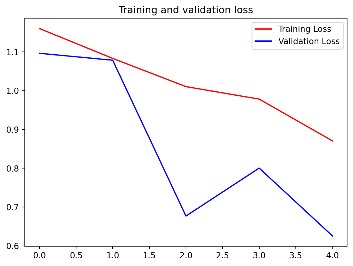
 1/20 ━━━━━━━━━━━━━━━━━━━━ 2:08 7s/step - accuracy: 0.4841 - loss: 1.0897 2/20 ━━━━━━━━━━━━━━━━━━━━ 33s 2s/step - accuracy: 0.4583 - loss: 1.0807  3/20 ━━━━━━━━━━━━━━━━━━━━ 29s 2s/step - accuracy: 0.4625 - loss: 1.0633 4/20 ━━━━━━━━━━━━━━━━━━━━ 27s 2s/step - accuracy: 0.4669 - loss: 1.0455 5/20 ━━━━━━━━━━━━━━━━━━━━ 26s 2s/step - accuracy: 0.4745 - loss: 1.0306 6/20 ━━━━━━━━━━━━━━━━━━━━ 25s 2s/step - accuracy: 0.4829 - loss: 1.0173 7/20 ━━━━━━━━━━━━━━━━━━━━ 23s 2s/step - accuracy: 0.4906 - loss: 1.0040 8/20 ━━━━━━━━━━━━━━━━━━━━ 21s 2s/step - accuracy: 0.4968 - loss: 0.9926 9/20 ━━━━━━━━━━━━━━━━━━━━ 19s 2s/step - accuracy: 0.5032 - loss: 0.982110/20 ━━━━━━━━━━━━━━━━━━━━ 17s 2s/step - accuracy: 0.5090 - loss: 0.973111/20 ━━━━━━━━━━━━━━━━━━━━ 15s 2s/step - accuracy: 0.5144 - loss: 0.965712/20 ━━━━━━━━━━━━━━━━━━━━ 13s 2s/step - accuracy: 0.5201 - loss: 0.959113/20 ━━━━━━━━━━━━━━━━━━━━ 12s 2s/step - accuracy: 0.5246 - loss: 0.953614/20 ━━━━━━━━━━━━━━━━━━━━ 10s 2s/step - accuracy: 0.5274 - loss: 0.951215/20 ━━━━━━━━━━━━━━━━━━━━ 8s 2s/step - accuracy: 0.5305 - loss: 0.9486 16/20 ━━━━━━━━━━━━━━━━━━━━ 6s 2s/step - accuracy: 0.5338 - loss: 0.945717/20 ━━━━━━━━━━━━━━━━━━━━ 5s 2s/step - accuracy: 0.5371 - loss: 0.942618/20 ━━━━━━━━━━━━━━━━━━━━ 3s 2s/step - accuracy: 0.5401 - loss: 0.939219/20 ━━━━━━━━━━━━━━━━━━━━ 1s 2s/step - accuracy: 0.5429 - loss: 0.935720/20 ━━━━━━━━━━━━━━━━━━━━ 0s 2s/step - accuracy: 0.5456 - loss: 0.932520/20 ━━━━━━━━━━━━━━━━━━━━ 40s 2s/step - accuracy: 0.5479 - loss: 0.9295 - val_accuracy: 0.8011 - val_loss: 0.6255

Code

acc = history.history['accuracy']
val_acc = history.history['val_accuracy']
loss = history.history['loss']
val_loss = history.history['val_loss']
epochs = range(len(acc))

Code

import matplotlib.image as mpimg
import matplotlib.pyplot as plt
#------------------------------------------------
# Plot training and validation accuracy per epoch
#------------------------------------------------
plt.plot(epochs, acc, 'r', label='Training accuracy')
plt.plot(epochs, val_acc, 'b', label='Validation accuracy')
plt.title('Training and validation accuracy')

plt.figure()

plt.plot(epochs, loss, 'r', label='Training Loss')
plt.plot(epochs, val_loss, 'b', label='Validation Loss')
plt.title('Training and validation loss')
plt.legend()

plt.show()

7 save model

Code

# Save the entire model as a `.keras` zip archive.
model.save('c2week4_rock_paper_scissors.keras')

8 load model

Code

new_model = tf.keras.models.load_model('c2week4_rock_paper_scissors.keras')

Code

new_model.summary()

Model: "sequential"

┏━━━━━━━━━━━━━━━━━━━━━━━━━━━━━━━━━┳━━━━━━━━━━━━━━━━━━━━━━━━┳━━━━━━━━━━━━━━━┓
┃ Layer (type)                    ┃ Output Shape           ┃       Param # ┃
┡━━━━━━━━━━━━━━━━━━━━━━━━━━━━━━━━━╇━━━━━━━━━━━━━━━━━━━━━━━━╇━━━━━━━━━━━━━━━┩
│ conv2d (Conv2D)                 │ (None, 148, 148, 64)   │         1,792 │
├─────────────────────────────────┼────────────────────────┼───────────────┤
│ max_pooling2d (MaxPooling2D)    │ (None, 74, 74, 64)     │             0 │
├─────────────────────────────────┼────────────────────────┼───────────────┤
│ conv2d_1 (Conv2D)               │ (None, 72, 72, 64)     │        36,928 │
├─────────────────────────────────┼────────────────────────┼───────────────┤
│ max_pooling2d_1 (MaxPooling2D)  │ (None, 36, 36, 64)     │             0 │
├─────────────────────────────────┼────────────────────────┼───────────────┤
│ conv2d_2 (Conv2D)               │ (None, 34, 34, 128)    │        73,856 │
├─────────────────────────────────┼────────────────────────┼───────────────┤
│ max_pooling2d_2 (MaxPooling2D)  │ (None, 17, 17, 128)    │             0 │
├─────────────────────────────────┼────────────────────────┼───────────────┤
│ conv2d_3 (Conv2D)               │ (None, 15, 15, 128)    │       147,584 │
├─────────────────────────────────┼────────────────────────┼───────────────┤
│ max_pooling2d_3 (MaxPooling2D)  │ (None, 7, 7, 128)      │             0 │
├─────────────────────────────────┼────────────────────────┼───────────────┤
│ flatten (Flatten)               │ (None, 6272)           │             0 │
├─────────────────────────────────┼────────────────────────┼───────────────┤
│ dropout (Dropout)               │ (None, 6272)           │             0 │
├─────────────────────────────────┼────────────────────────┼───────────────┤
│ dense (Dense)                   │ (None, 512)            │     3,211,776 │
├─────────────────────────────────┼────────────────────────┼───────────────┤
│ dense_1 (Dense)                 │ (None, 3)              │         1,539 │
└─────────────────────────────────┴────────────────────────┴───────────────┘

 Total params: 6,946,952 (26.50 MB)

 Trainable params: 3,473,475 (13.25 MB)

 Non-trainable params: 0 (0.00 B)

 Optimizer params: 3,473,477 (13.25 MB)

9 resource:

https://coursera.org/learn/convolutional-neural-networks-tensorflow/home/

https://github.com/https-deeplearning-ai/tensorflow-1-public/tree/main/C2

https://www.kaggle.com/c/dogs-vs-cats