Code
import tensorflow as tf
import numpy as np
import matplotlib.pyplot as pltWeek 1 Sequences and Prediction
Hi Learners and welcome to this course on sequences and prediction! In this course we’ll take a look at some of the unique considerations involved when handling sequential time series data – where values change over time, like the temperature on a particular day, or the number of visitors to your web site. We’ll discuss various methodologies for predicting future values in these time series, building on what you’ve learned in previous courses!
what exactly is a time series?
It’s typically defined as an ordered sequence of values that are usually equally spaced over time
import tensorflow as tf
import numpy as np
import matplotlib.pyplot as plt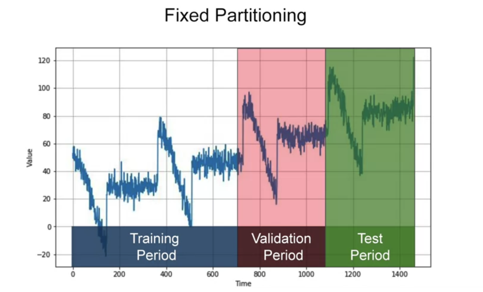
def plot_series(time, series, format="-", start=0, end=None):
    """
    Visualizes time series data

    Args:
      time (array of int) - contains the time steps
      series (array of int) - contains the measurements for each time step
      format - line style when plotting the graph
      label - tag for the line
      start - first time step to plot
      end - last time step to plot
    """

    # Setup dimensions of the graph figure
    plt.figure(figsize=(10, 6))

    if type(series) is tuple:

      for series_num in series:
        # Plot the time series data
        plt.plot(time[start:end], series_num[start:end], format)

    else:
      # Plot the time series data
      plt.plot(time[start:end], series[start:end], format)

    # Label the x-axis
    plt.xlabel("Time")

    # Label the y-axis
    plt.ylabel("Value")

    # Overlay a grid on the graph
    plt.grid(True)

    # Draw the graph on screen
plt.show()def trend(time, slope=0):
"""
Generates synthetic data that follows a straight line given a slope value.
Args:
time (array of int) - contains the time steps
slope (float) - determines the direction and steepness of the line
Returns:
series (array of float) - measurements that follow a straight line
"""
# Compute the linear series given the slope
series = slope * time
return series
def seasonal_pattern(season_time):
"""
Just an arbitrary pattern, you can change it if you wish
Args:
season_time (array of float) - contains the measurements per time step
Returns:
data_pattern (array of float) - contains revised measurement values according
to the defined pattern
"""
# Generate the values using an arbitrary pattern
data_pattern = np.where(season_time < 0.4,
np.cos(season_time * 2 * np.pi),
1 / np.exp(3 * season_time))
return data_pattern
def seasonality(time, period, amplitude=1, phase=0):
"""
Repeats the same pattern at each period
Args:
time (array of int) - contains the time steps
period (int) - number of time steps before the pattern repeats
amplitude (int) - peak measured value in a period
phase (int) - number of time steps to shift the measured values
Returns:
data_pattern (array of float) - seasonal data scaled by the defined amplitude
"""
# Define the measured values per period
season_time = ((time + phase) % period) / period
# Generates the seasonal data scaled by the defined amplitude
data_pattern = amplitude * seasonal_pattern(season_time)
return data_pattern
def noise(time, noise_level=1, seed=None):
"""Generates a normally distributed noisy signal
Args:
time (array of int) - contains the time steps
noise_level (float) - scaling factor for the generated signal
seed (int) - number generator seed for repeatability
Returns:
noise (array of float) - the noisy signal
"""
# Initialize the random number generator
rnd = np.random.RandomState(seed)
# Generate a random number for each time step and scale by the noise level
noise = rnd.randn(len(time)) * noise_level
return noise# Parameters
time = np.arange(4 * 365 + 1, dtype="float32")
baseline = 10
amplitude = 40
slope = 0.05
noise_level = 5
print(len(time))1461# Create the series
series = baseline + trend(time, slope) + seasonality(time, period=365, amplitude=amplitude)
# Update with noise
series = series+noise(time, noise_level, seed=42)
# Plot the results
plot_series(time, series)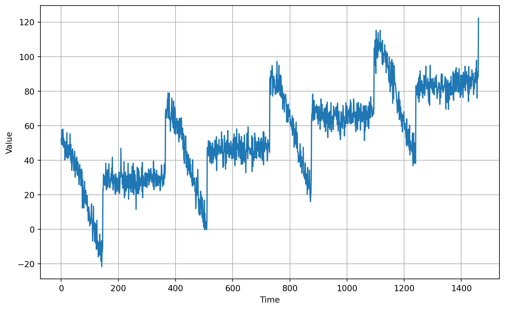
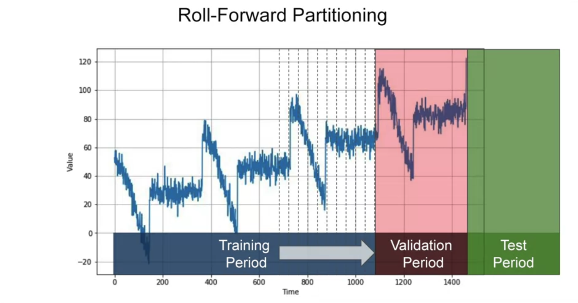
# Define the split time
split_time = 1000

# Get the train set
time_train = time[:split_time]
x_train = series[:split_time]

# Get the validation set
time_valid = time[split_time:]
x_valid = series[split_time:]
1 to 1000 for training
# Plot the train set
plot_series(time_train, x_train)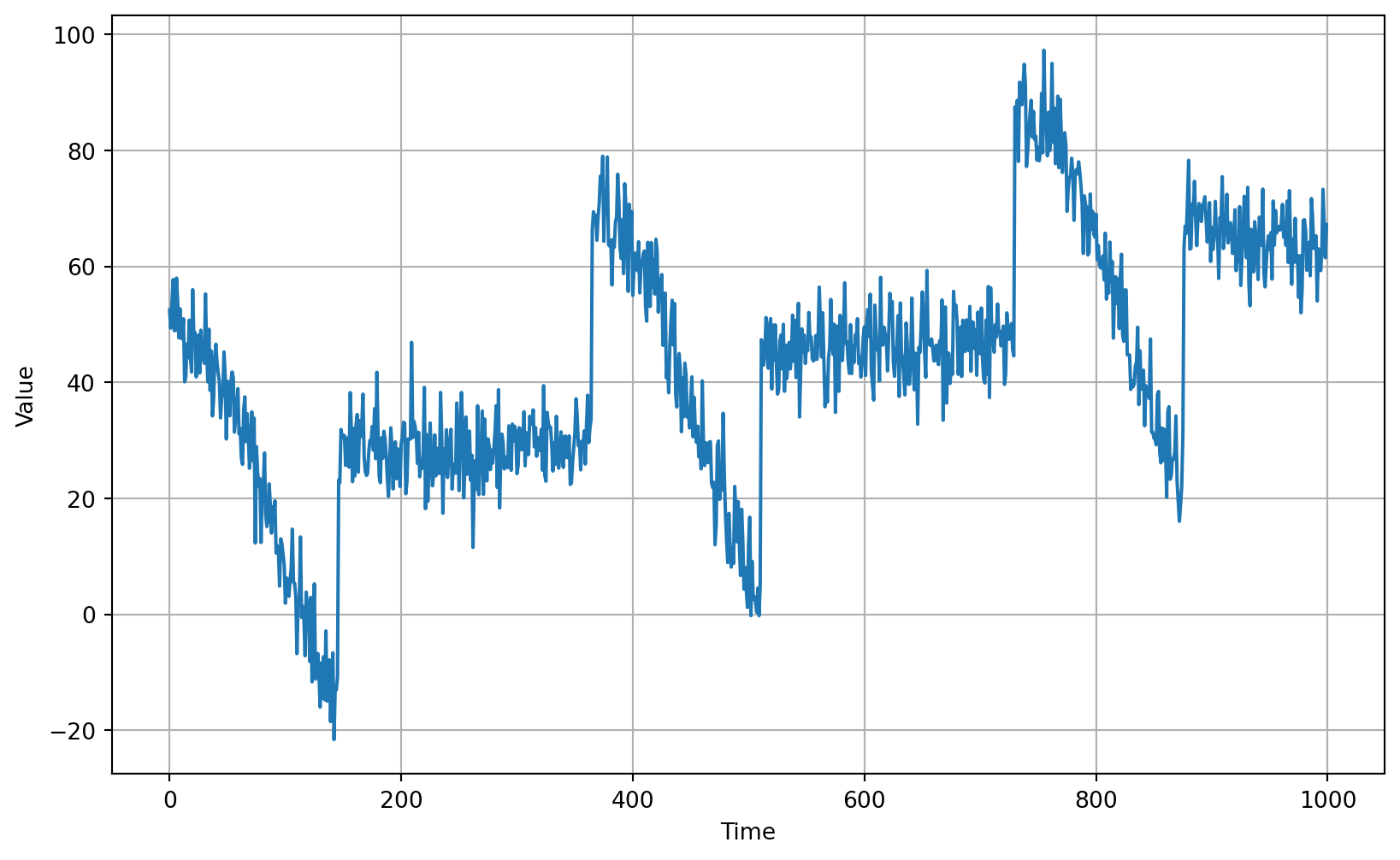
1000 to 1400 for valid
# Plot the validation set
plot_series(time_valid, x_valid)
naive_forecast = series[split_time - 1:-1]

# Define time step
time_step = 100

# Print values
print(f'ground truth at time step {time_step}: {x_valid[time_step]}')
print(f'prediction at time step {time_step + 1}: {naive_forecast[time_step + 1]}')
ground truth at time step 100: 109.84197926023576
prediction at time step 101: 109.84197926023576# Plot the results
plot_series(time_valid, (x_valid, naive_forecast))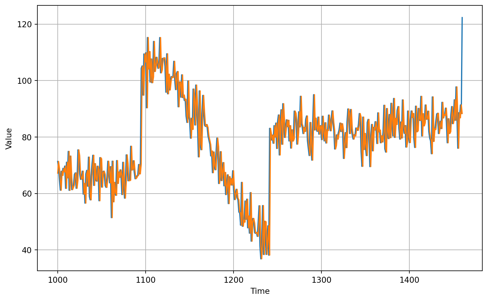
# Zooming in
plot_series(time_valid, (x_valid, naive_forecast), start=0, end=150)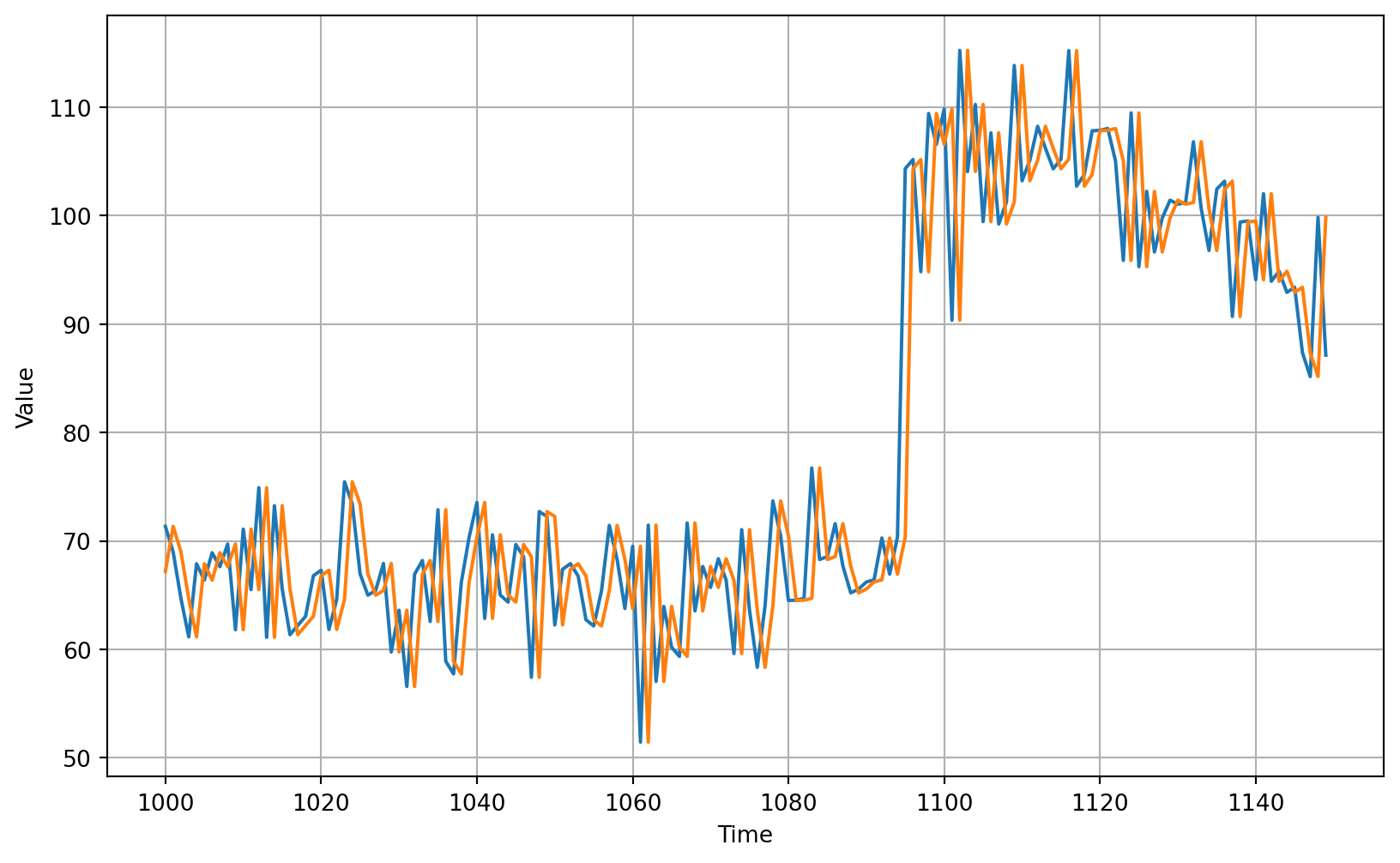
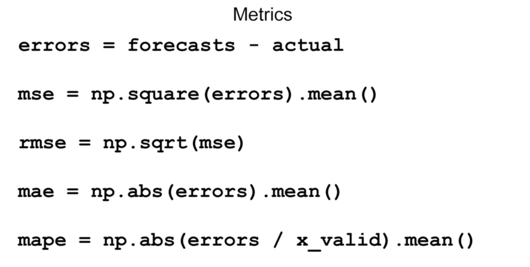
Computing Metrics
mean_squared_error:
print(tf.keras.metrics.mean_squared_error(x_valid, naive_forecast).numpy())61.8275342640202mean_absolute_error:
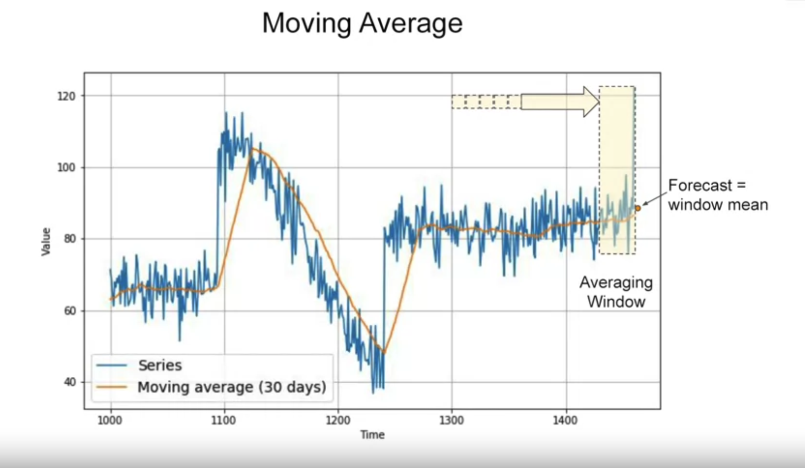
print(tf.keras.metrics.mean_absolute_error(x_valid, naive_forecast).numpy())5.9379084434271485def moving_average_forecast(series, window_size):
"""Generates a moving average forecast
Args:
series (array of float) - contains the values of the time series
window_size (int) - the number of time steps to compute the average for
Returns:
forecast (array of float) - the moving average forecast
"""
# Initialize a list
forecast = []
# Compute the moving average based on the window size
for time in range(len(series) - window_size):
forecast.append(series[time:time + window_size].mean())
# Convert to a numpy array
forecast = np.array(forecast)
return forecastusing past 30 day moving average
# Generate the moving average forecast
moving_avg = moving_average_forecast(series, 30)[split_time - 30:]

# Plot the results
plot_series(time_valid, (x_valid, moving_avg))
# Compute the metrics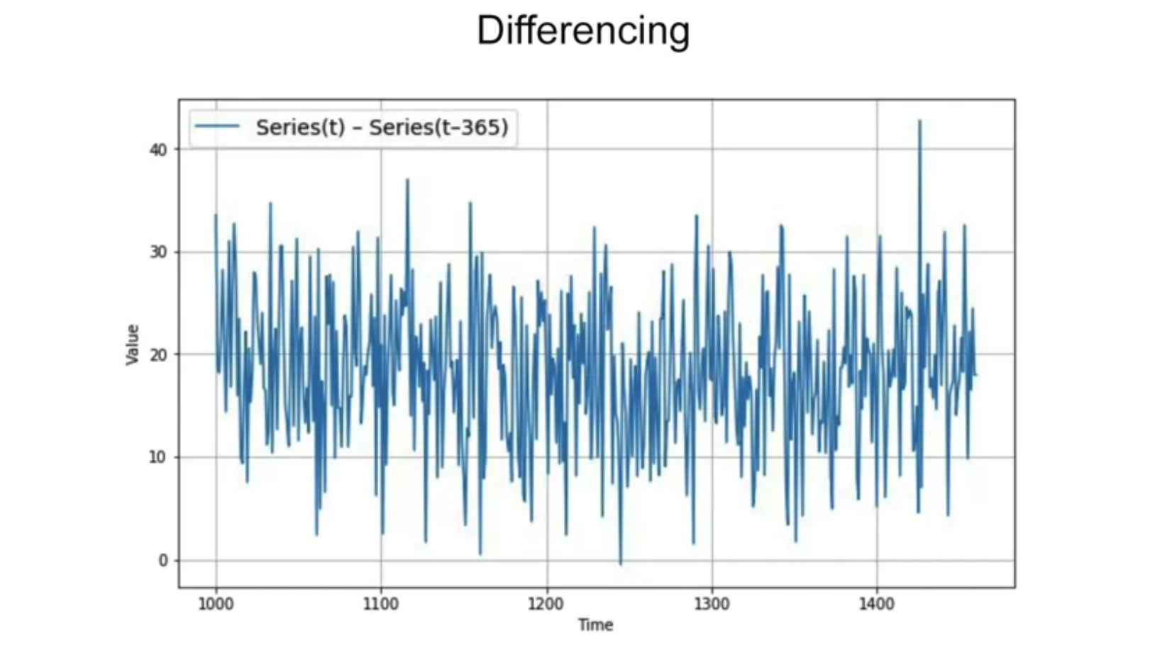
print(tf.keras.metrics.mean_squared_error(x_valid, moving_avg).numpy())106.67456927078204print(tf.keras.metrics.mean_absolute_error(x_valid, moving_avg).numpy())7.142418746782468365 days Differencing
# Subtract the values at t-365 from original series
diff_series = (series[365:] - series[:-365])

# Truncate the first 365 time steps
diff_time = time[365:]

# Plot the results
plot_series(diff_time, diff_series)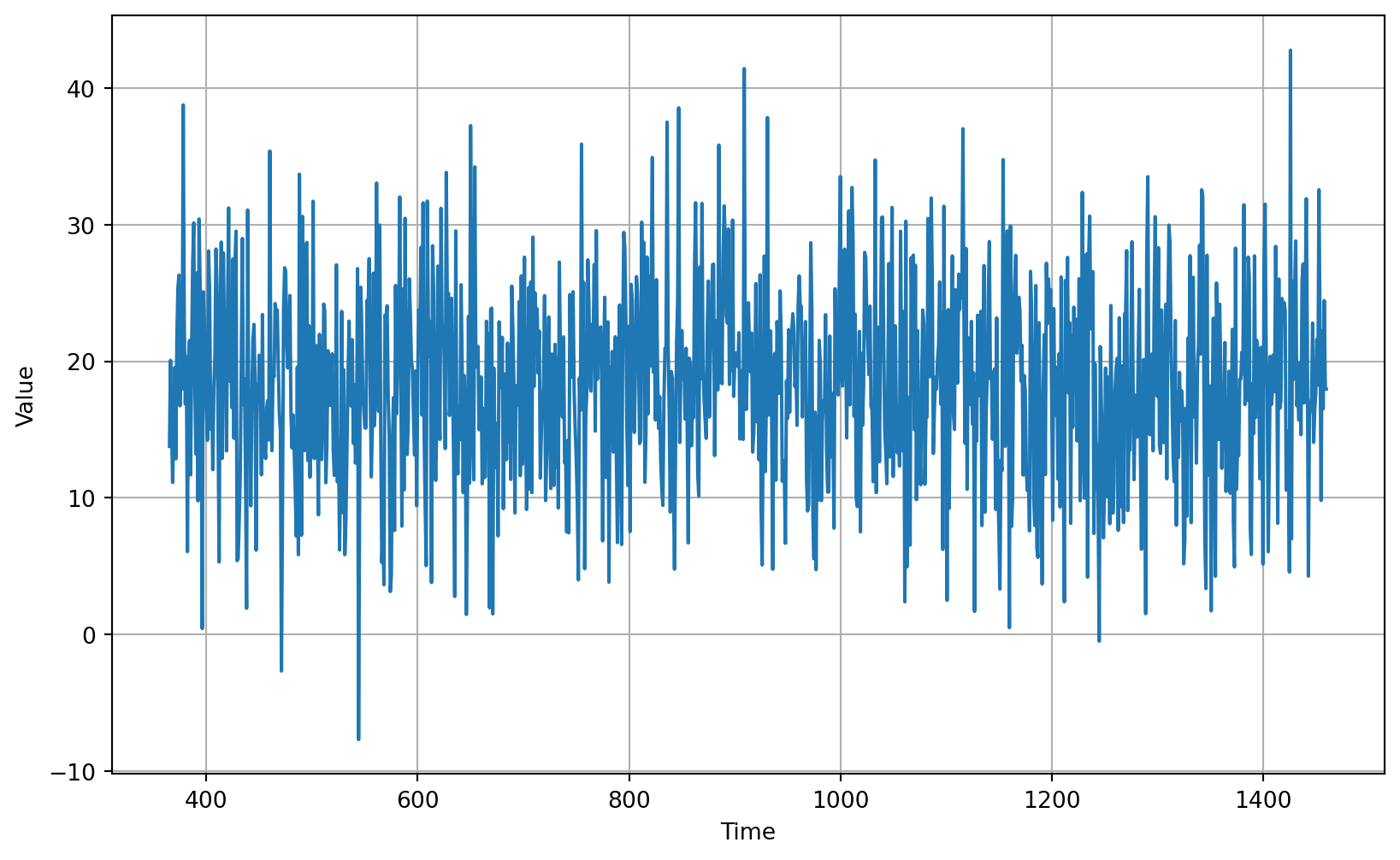
# Generate moving average from the time differenced dataset
diff_moving_avg = moving_average_forecast(diff_series, 30)

# Slice the prediction points that corresponds to the validation set time steps
diff_moving_avg = diff_moving_avg[split_time - 365 - 30:]

# Slice the ground truth points that corresponds to the validation set time steps
diff_series = diff_series[split_time - 365:]

# Plot the results
plot_series(time_valid, (diff_series, diff_moving_avg))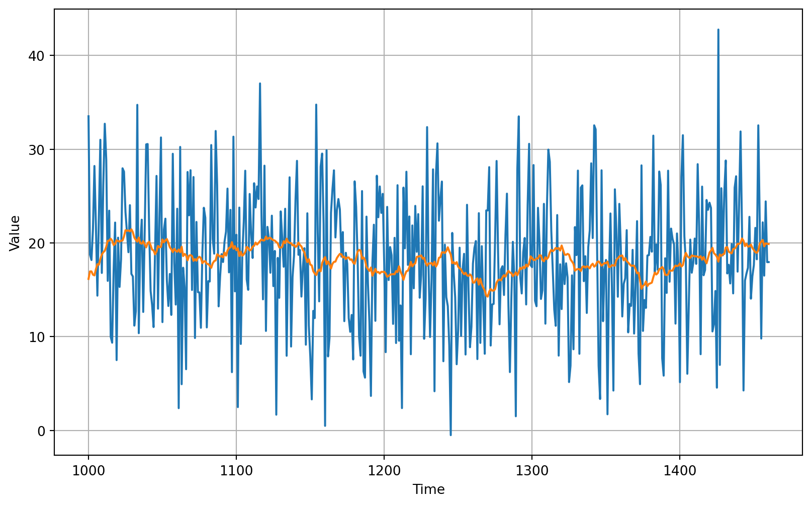
add back Differencing
# Add the trend and seasonality from the original series
diff_moving_avg_plus_past = series[split_time - 365:-365] + diff_moving_avg

# Plot the results
plot_series(time_valid, (x_valid, diff_moving_avg_plus_past))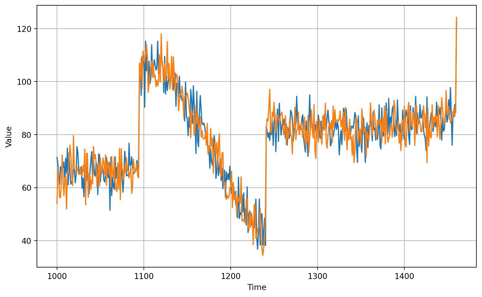
# Compute the metrics
print(tf.keras.metrics.mean_squared_error(x_valid, diff_moving_avg_plus_past).numpy())53.76458170166675print(tf.keras.metrics.mean_absolute_error(x_valid, diff_moving_avg_plus_past).numpy())5.903241526511199moving average with 11 days after remove referencing
# Smooth the original series before adding the time differenced moving average
diff_moving_avg_plus_smooth_past = moving_average_forecast(series[split_time - 370:-359], 11) + diff_moving_avg

# Plot the results
plot_series(time_valid, (x_valid, diff_moving_avg_plus_smooth_past))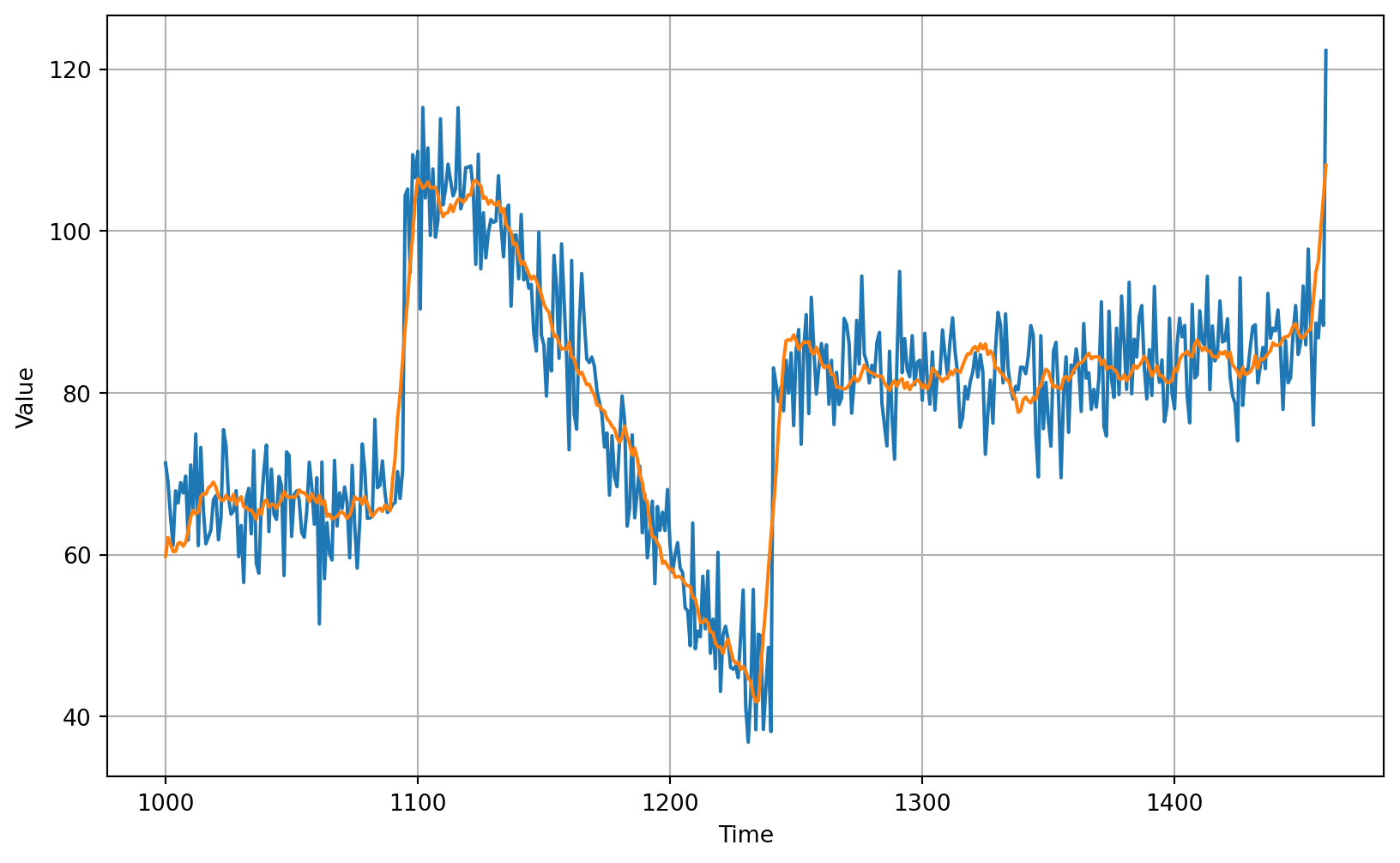
 # Compute the metrics
print(tf.keras.metrics.mean_squared_error(x_valid, diff_moving_avg_plus_smooth_past).numpy())34.3157226871993print(tf.keras.metrics.mean_absolute_error(x_valid, diff_moving_avg_plus_smooth_past).numpy())4.605328954146046https://www.coursera.org/learn/tensorflow-sequences-time-series-and-prediction
https://github.com/https-deeplearning-ai/tensorflow-1-public/tree/main/C4