W2:Deep Neural Networks for Time Series

Week 2 Deep Neural Networks for Time Series

Having explored time series and some of the common attributes of time series such as trend and seasonality, and then having used statistical methods for projection, let’s now begin to teach neural networks to recognize and predict on time series!

import tensorflow as tf

1 Create a Simple Dataset

# Generate a tf dataset with 10 elements (i.e. numbers 0 to 9)
dataset = tf.data.Dataset.range(10)

# Preview the result
for val in dataset:
   print(val)

tf.Tensor(0, shape=(), dtype=int64)
tf.Tensor(1, shape=(), dtype=int64)
tf.Tensor(2, shape=(), dtype=int64)
tf.Tensor(3, shape=(), dtype=int64)
tf.Tensor(4, shape=(), dtype=int64)
tf.Tensor(5, shape=(), dtype=int64)
tf.Tensor(6, shape=(), dtype=int64)
tf.Tensor(7, shape=(), dtype=int64)
tf.Tensor(8, shape=(), dtype=int64)
tf.Tensor(9, shape=(), dtype=int64)

2 Windowing the data

# Generate a tf dataset with 10 elements (i.e. numbers 0 to 9)
dataset = tf.data.Dataset.range(10)

# Window the data but only take those with the specified size
dataset = dataset.window(size=5, shift=1, drop_remainder=True)

# Print the result
for window_dataset in dataset:
  print([item.numpy() for item in window_dataset])

[0, 1, 2, 3, 4]
[1, 2, 3, 4, 5]
[2, 3, 4, 5, 6]
[3, 4, 5, 6, 7]
[4, 5, 6, 7, 8]
[5, 6, 7, 8, 9]

3 Flatten the Windows

# Generate a tf dataset with 10 elements (i.e. numbers 0 to 9)
dataset = tf.data.Dataset.range(10)

# Window the data but only take those with the specified size
dataset = dataset.window(5, shift=1, drop_remainder=True)

# Flatten the windows by putting its elements in a single batch
dataset = dataset.flat_map(lambda window: window.batch(5))

# Print the results
for window in dataset:
  print(window.numpy())

[0 1 2 3 4]
[1 2 3 4 5]
[2 3 4 5 6]
[3 4 5 6 7]
[4 5 6 7 8]
[5 6 7 8 9]

4 Group into features and labels

# Generate a tf dataset with 10 elements (i.e. numbers 0 to 9)
dataset = tf.data.Dataset.range(10)

# Window the data but only take those with the specified size
dataset = dataset.window(5, shift=1, drop_remainder=True)

# Flatten the windows by putting its elements in a single batch
dataset = dataset.flat_map(lambda window: window.batch(5))

# Create tuples with features (first four elements of the window) and labels (last element)
dataset = dataset.map(lambda window: (window[:-1], window[-1]))

# Print the results
for x,y in dataset:
  print("x = ", x.numpy())
  print("y = ", y.numpy())
  print()

x =  [0 1 2 3]
y =  4

x =  [1 2 3 4]
y =  5

x =  [2 3 4 5]
y =  6

x =  [3 4 5 6]
y =  7

x =  [4 5 6 7]
y =  8

x =  [5 6 7 8]
y =  9

5 Shuffle the data

# Generate a tf dataset with 10 elements (i.e. numbers 0 to 9)
dataset = tf.data.Dataset.range(10)

# Window the data but only take those with the specified size
dataset = dataset.window(5, shift=1, drop_remainder=True)

# Flatten the windows by putting its elements in a single batch
dataset = dataset.flat_map(lambda window: window.batch(5))

# Create tuples with features (first four elements of the window) and labels (last element)
dataset = dataset.map(lambda window: (window[:-1], window[-1]))

# Shuffle the windows
dataset = dataset.shuffle(buffer_size=10)

# Print the results
for x,y in dataset:
  print("x = ", x.numpy())
  print("y = ", y.numpy())
  print()

x =  [1 2 3 4]
y =  5

x =  [4 5 6 7]
y =  8

x =  [0 1 2 3]
y =  4

x =  [3 4 5 6]
y =  7

x =  [2 3 4 5]
y =  6

x =  [5 6 7 8]
y =  9

6 Create batches for training

# Generate a tf dataset with 10 elements (i.e. numbers 0 to 9)
dataset = tf.data.Dataset.range(10)

# Window the data but only take those with the specified size
dataset = dataset.window(5, shift=1, drop_remainder=True)

# Flatten the windows by putting its elements in a single batch
dataset = dataset.flat_map(lambda window: window.batch(5))

# Create tuples with features (first four elements of the window) and labels (last element)
dataset = dataset.map(lambda window: (window[:-1], window[-1]))

# Shuffle the windows
dataset = dataset.shuffle(buffer_size=10)

# Create batches of windows
dataset = dataset.batch(2).prefetch(1)

# Print the results
for x,y in dataset:
  print("x = ", x.numpy())
  print("y = ", y.numpy())
  print()

x =  [[0 1 2 3]
 [5 6 7 8]]
y =  [4 9]

x =  [[3 4 5 6]
 [1 2 3 4]]
y =  [7 5]

x =  [[2 3 4 5]
 [4 5 6 7]]
y =  [6 8]

7 Utilities

import tensorflow as tf
import numpy as np
import matplotlib.pyplot as plt

def plot_series(time, series, format="-", start=0, end=None):
    """
    Visualizes time series data

    Args:
      time (array of int) - contains the time steps
      series (array of int) - contains the measurements for each time step
      format - line style when plotting the graph
      label - tag for the line
      start - first time step to plot
      end - last time step to plot
    """

    # Setup dimensions of the graph figure
    plt.figure(figsize=(10, 6))
    
    if type(series) is tuple:

      for series_num in series:
        # Plot the time series data
        plt.plot(time[start:end], series_num[start:end], format)

    else:
      # Plot the time series data
      plt.plot(time[start:end], series[start:end], format)

    # Label the x-axis
    plt.xlabel("Time")

    # Label the y-axis
    plt.ylabel("Value")

    # Overlay a grid on the graph
    plt.grid(True)

    # Draw the graph on screen
    plt.show()


def trend(time, slope=0):
    """
    Generates synthetic data that follows a straight line given a slope value.

    Args:
      time (array of int) - contains the time steps
      slope (float) - determines the direction and steepness of the line

    Returns:
      series (array of float) - measurements that follow a straight line
    """

    # Compute the linear series given the slope
    series = slope * time

    return series


def seasonal_pattern(season_time):
    """
    Just an arbitrary pattern, you can change it if you wish
    
    Args:
      season_time (array of float) - contains the measurements per time step

    Returns:
      data_pattern (array of float) -  contains revised measurement values according 
                                  to the defined pattern
    """

    # Generate the values using an arbitrary pattern
    data_pattern = np.where(season_time < 0.4,
                    np.cos(season_time * 2 * np.pi),
                    1 / np.exp(3 * season_time))
    
    return data_pattern


def seasonality(time, period, amplitude=1, phase=0):
    """
    Repeats the same pattern at each period

    Args:
      time (array of int) - contains the time steps
      period (int) - number of time steps before the pattern repeats
      amplitude (int) - peak measured value in a period
      phase (int) - number of time steps to shift the measured values

    Returns:
      data_pattern (array of float) - seasonal data scaled by the defined amplitude
    """
    
    # Define the measured values per period
    season_time = ((time + phase) % period) / period

    # Generates the seasonal data scaled by the defined amplitude
    data_pattern = amplitude * seasonal_pattern(season_time)

    return data_pattern


def noise(time, noise_level=1, seed=None):
    """Generates a normally distributed noisy signal

    Args:
      time (array of int) - contains the time steps
      noise_level (float) - scaling factor for the generated signal
      seed (int) - number generator seed for repeatability

    Returns:
      noise (array of float) - the noisy signal
    """

    # Initialize the random number generator
    rnd = np.random.RandomState(seed)

    # Generate a random number for each time step and scale by the noise level
    noise = rnd.randn(len(time)) * noise_level
    
    return noise

8 Generate the Synthetic Data

# Parameters
time = np.arange(4 * 365 + 1, dtype="float32")
baseline = 10
amplitude = 40
slope = 0.05
noise_level = 5

# Create the series
series = baseline + trend(time, slope) + seasonality(time, period=365, amplitude=amplitude)

# Update with noise
series += noise(time, noise_level, seed=42)

# Plot the results
plot_series(time, series)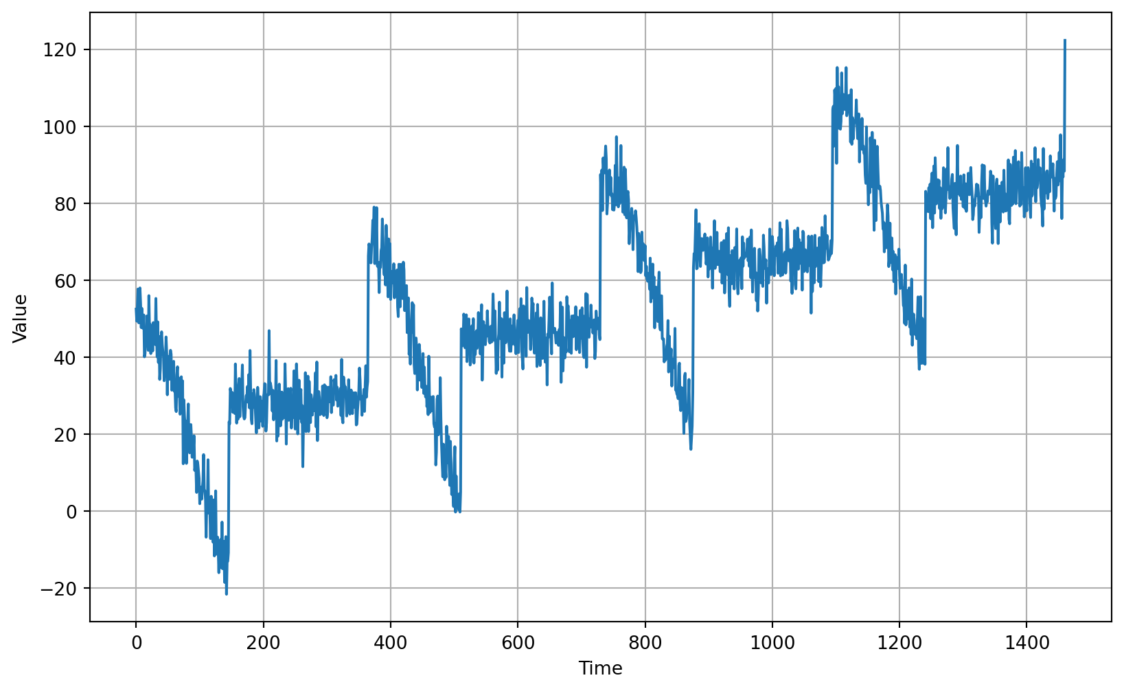

9 Split the Dataset

# Define the split time
split_time = 1000

# Get the train set 
time_train = time[:split_time]
x_train = series[:split_time]

# Get the validation set
time_valid = time[split_time:]
x_valid = series[split_time:]

# Plot the train set
plot_series(time_train, x_train)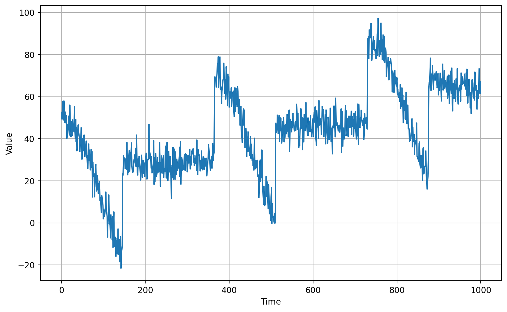

# Plot the validation set
plot_series(time_valid, x_valid)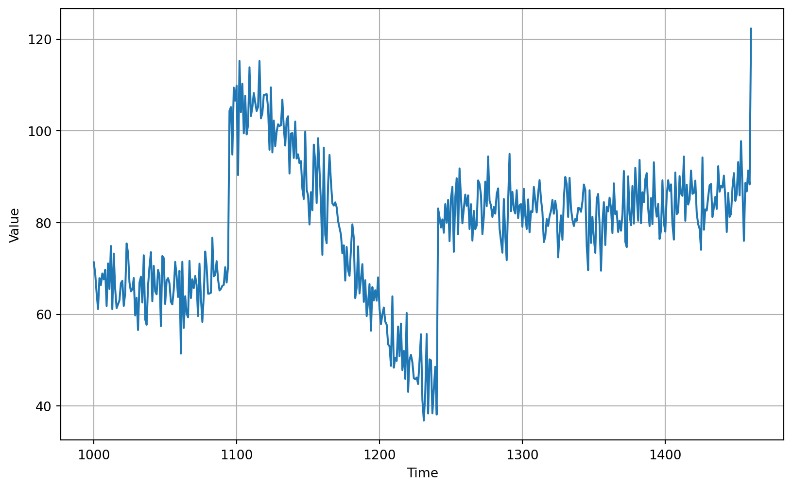

10 Prepare features and labels

using 20 day window

# Parameters
window_size = 20
batch_size = 32
shuffle_buffer_size = 1000

def windowed_dataset(series, window_size, batch_size, shuffle_buffer):
    """Generates dataset windows

    Args:
      series (array of float) - contains the values of the time series
      window_size (int) - the number of time steps to include in the feature
      batch_size (int) - the batch size
      shuffle_buffer(int) - buffer size to use for the shuffle method

    Returns:
      dataset (TF Dataset) - TF Dataset containing time windows
    """
  
    # Generate a TF Dataset from the series values
    dataset = tf.data.Dataset.from_tensor_slices(series)
    
    # Window the data but only take those with the specified size
    dataset = dataset.window(window_size + 1, shift=1, drop_remainder=True)
    
    # Flatten the windows by putting its elements in a single batch
    dataset = dataset.flat_map(lambda window: window.batch(window_size + 1))

    # Create tuples with features and labels 
    dataset = dataset.map(lambda window: (window[:-1], window[-1]))

    # Shuffle the windows
    dataset = dataset.shuffle(shuffle_buffer)
    
    # Create batches of windows
    dataset = dataset.batch(batch_size).prefetch(1)
    
    return dataset

# Generate the dataset windows
dataset = windowed_dataset(x_train, window_size, batch_size, shuffle_buffer_size)

# Print properties of a single batch
for windows in dataset.take(1):
  print(f'data type: {type(windows)}')
  print(f'number of elements in the tuple: {len(windows)}')
  print(f'shape of first element: {windows[0].shape}')
  print(f'shape of second element: {windows[1].shape}')

data type: <class 'tuple'>
number of elements in the tuple: 2
shape of first element: (32, 20)
shape of second element: (32,)

11 define single layer neural model

# Build the single layer neural network
l0 = tf.keras.layers.Dense(1, input_shape=[window_size])
model = tf.keras.models.Sequential([l0])

# Print the initial layer weights
print("Layer weights: \n {} \n".format(l0.get_weights()))

# Print the model summary
model.summary()

Layer weights: 
 [array([[-0.02897543],
       [ 0.2368316 ],
       [-0.4459325 ],
       [-0.00241488],
       [ 0.48065752],
       [-0.48599264],
       [ 0.51217467],
       [-0.01346123],
       [ 0.09258026],
       [ 0.14586818],
       [ 0.3576712 ],
       [-0.5222965 ],
       [ 0.28616023],
       [ 0.14155024],
       [ 0.09476584],
       [ 0.2801147 ],
       [ 0.07839262],
       [-0.22657192],
       [ 0.10993838],
       [ 0.1691292 ]], dtype=float32), array([0.], dtype=float32)] 

Model: "sequential"

┏━━━━━━━━━━━━━━━━━━━━━━━━━━━━━━━━━┳━━━━━━━━━━━━━━━━━━━━━━━━┳━━━━━━━━━━━━━━━┓
┃ Layer (type)                    ┃ Output Shape           ┃       Param # ┃
┡━━━━━━━━━━━━━━━━━━━━━━━━━━━━━━━━━╇━━━━━━━━━━━━━━━━━━━━━━━━╇━━━━━━━━━━━━━━━┩
│ dense (Dense)                   │ (None, 1)              │            21 │
└─────────────────────────────────┴────────────────────────┴───────────────┘

 Total params: 21 (84.00 B)

 Trainable params: 21 (84.00 B)

 Non-trainable params: 0 (0.00 B)

12 compile model

# Set the training parameters
model.compile(loss="mse", optimizer=tf.keras.optimizers.SGD(learning_rate=1e-6, momentum=0.9))

13 Train the Model

# Train the model
model.fit(dataset,epochs=100,verbose=0)

<keras.src.callbacks.history.History at 0x14d7921d0>

# Print the layer weights
print("Layer weights {}".format(l0.get_weights()))

Layer weights [array([[-0.02693498],
       [ 0.02551215],
       [-0.03809907],
       [-0.02330507],
       [ 0.1171276 ],
       [-0.10470365],
       [ 0.07021185],
       [-0.03254524],
       [-0.00710663],
       [ 0.01842318],
       [ 0.057825  ],
       [-0.12609479],
       [ 0.014718  ],
       [ 0.03457457],
       [ 0.0259654 ],
       [ 0.07261312],
       [ 0.04803773],
       [ 0.10154756],
       [ 0.30292708],
       [ 0.44251084]], dtype=float32), array([0.01477173], dtype=float32)]

14 Model Prediction

# Shape of the first 20 data points slice
print(f'shape of series[0:20]: {series[0:20].shape}')

# Shape after adding a batch dimension
print(f'shape of series[0:20][np.newaxis]: {series[0:20][np.newaxis].shape}')

# Shape after adding a batch dimension (alternate way)
print(f'shape of series[0:20][np.newaxis]: {np.expand_dims(series[0:20], axis=0).shape}')

# Sample model prediction
print(f'model prediction: {model.predict(series[0:20][np.newaxis])}')

shape of series[0:20]: (20,)
shape of series[0:20][np.newaxis]: (1, 20)
shape of series[0:20][np.newaxis]: (1, 20)
1/1 ━━━━━━━━━━━━━━━━━━━━ 0s 14ms/step1/1 ━━━━━━━━━━━━━━━━━━━━ 0s 15ms/step
model prediction: [[42.610508]]

# Initialize a list
forecast = []

# Use the model to predict data points per window size
for time in range(len(series) - window_size):
  forecast.append(model.predict(series[time:time + window_size][np.newaxis]))

# Slice the points that are aligned with the validation set
forecast = forecast[split_time - window_size:]

# Compare number of elements in the predictions and the validation set
print(f'length of the forecast list: {len(forecast)}')
print(f'shape of the validation set: {x_valid.shape}')

length of the forecast list: 461
shape of the validation set: (461,)

# Preview shapes after using the conversion and squeeze methods
print(f'shape after converting to numpy array: {np.array(forecast).shape}')
print(f'shape after squeezing: {np.array(forecast).squeeze().shape}')

# Convert to a numpy array and drop single dimensional axes
results = np.array(forecast).squeeze()

# Overlay the results with the validation set
plot_series(time_valid, (x_valid, results))

shape after converting to numpy array: (461, 1, 1)
shape after squeezing: (461,)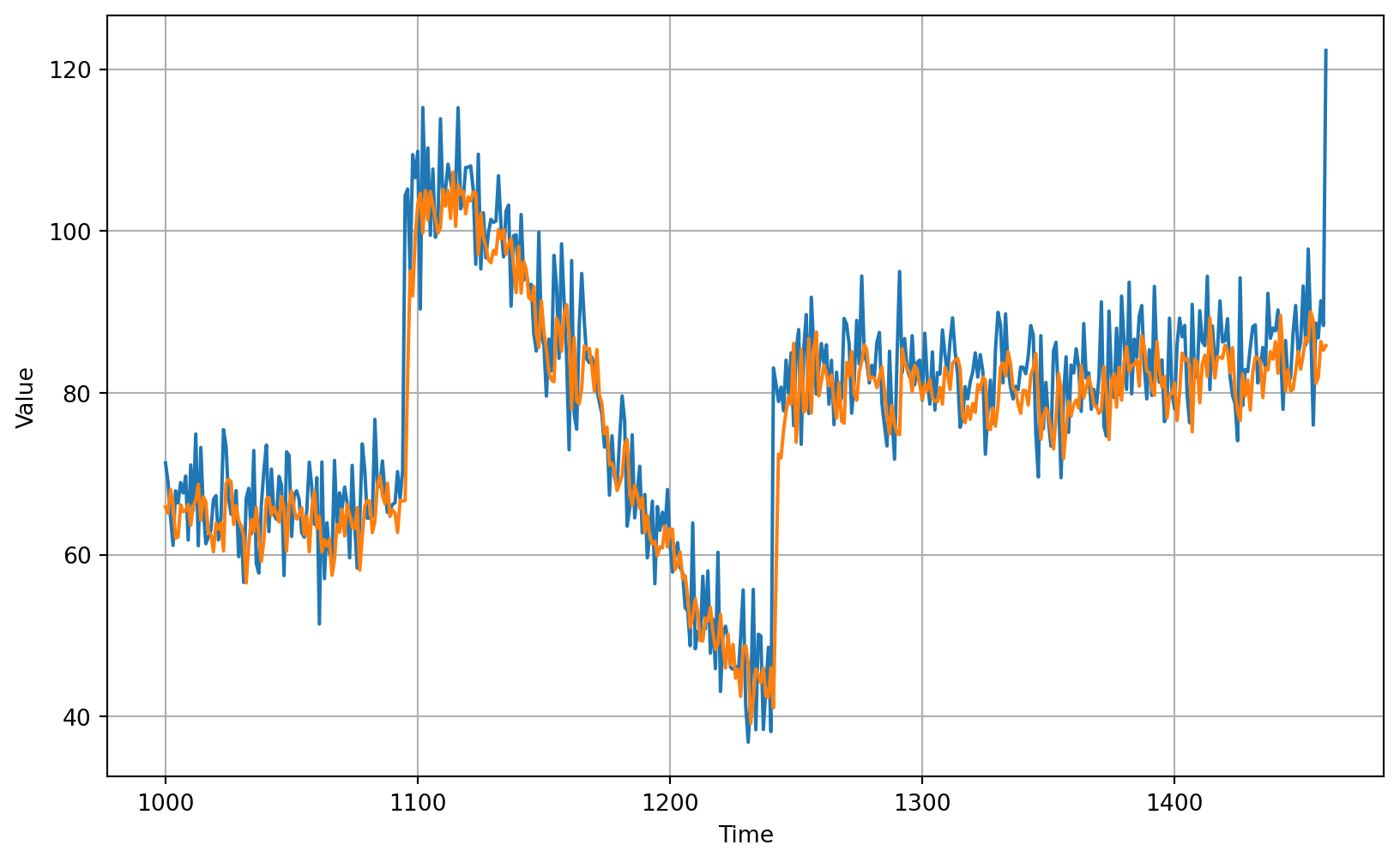

# Compute the metrics
print(tf.keras.metrics.mean_squared_error(x_valid, results).numpy())

50.470028

# Compute the metrics
print(tf.keras.metrics.mean_absolute_error(x_valid, results).numpy())

5.173313

15 DNN

# Generate the dataset windows
dataset = windowed_dataset(x_train, window_size, batch_size, shuffle_buffer_size)

16 # define DNN model

# Build the model
model_baseline = tf.keras.models.Sequential([
    tf.keras.layers.Dense(10, input_shape=[window_size], activation="relu"), 
    tf.keras.layers.Dense(10, activation="relu"), 
    tf.keras.layers.Dense(1)
])

# Print the model summary
model_baseline.summary()

Model: "sequential_1"

┏━━━━━━━━━━━━━━━━━━━━━━━━━━━━━━━━━┳━━━━━━━━━━━━━━━━━━━━━━━━┳━━━━━━━━━━━━━━━┓
┃ Layer (type)                    ┃ Output Shape           ┃       Param # ┃
┡━━━━━━━━━━━━━━━━━━━━━━━━━━━━━━━━━╇━━━━━━━━━━━━━━━━━━━━━━━━╇━━━━━━━━━━━━━━━┩
│ dense_1 (Dense)                 │ (None, 10)             │           210 │
├─────────────────────────────────┼────────────────────────┼───────────────┤
│ dense_2 (Dense)                 │ (None, 10)             │           110 │
├─────────────────────────────────┼────────────────────────┼───────────────┤
│ dense_3 (Dense)                 │ (None, 1)              │            11 │
└─────────────────────────────────┴────────────────────────┴───────────────┘

 Total params: 331 (1.29 KB)

 Trainable params: 331 (1.29 KB)

 Non-trainable params: 0 (0.00 B)

17 compile model

# Set the training parameters
model_baseline.compile(loss="mse", optimizer=tf.keras.optimizers.SGD(learning_rate=1e-6, momentum=0.9))

18 Train the Model

# Train the model
model_baseline.fit(dataset,epochs=100,verbose=0)

<keras.src.callbacks.history.History at 0x177b2df90>

19 result

# Initialize a list
forecast = []

# Reduce the original series
forecast_series = series[split_time - window_size:]

# Use the model to predict data points per window size
for time in range(len(forecast_series) - window_size):
  forecast.append(model_baseline.predict(forecast_series[time:time + window_size][np.newaxis]))

# Convert to a numpy array and drop single dimensional axes
results = np.array(forecast).squeeze()

# Plot the results
plot_series(time_valid, (x_valid, results))

# Compute the metrics
print(tf.keras.metrics.mean_squared_error(x_valid, results).numpy())

46.421417

print(tf.keras.metrics.mean_absolute_error(x_valid, results).numpy())

5.0056305

20 Tune the learning rate

clear

tf.keras.backend.clear_session()

21 define DNN model

# Build the Model
model_tune = tf.keras.models.Sequential([
    tf.keras.layers.Dense(10, input_shape=[window_size], activation="relu"), 
    tf.keras.layers.Dense(10, activation="relu"), 
    tf.keras.layers.Dense(1)
])

22 set callbacks for learning rate tunning

# Set the learning rate scheduler
lr_schedule = tf.keras.callbacks.LearningRateScheduler(
    lambda epoch: 1e-8 * 10**(epoch / 20))

23 complie model

# Initialize the optimizer
optimizer = tf.keras.optimizers.SGD(momentum=0.9)

# Set the training parameters
model_tune.compile(loss="mse", optimizer=optimizer)

24 train model

# Train the model
history = model_tune.fit(dataset, epochs=100, callbacks=[lr_schedule],verbose=0)

# Define the learning rate array
lrs = 1e-8 * (10 ** (np.arange(100) / 20))

# Set the figure size
plt.figure(figsize=(10, 6))

# Set the grid
plt.grid(True)

# Plot the loss in log scale
plt.semilogx(lrs, history.history["loss"])

# Increase the tickmarks size
plt.tick_params('both', length=10, width=1, which='both')

# Set the plot boundaries
plt.axis([1e-8, 1e-3, 0, 300])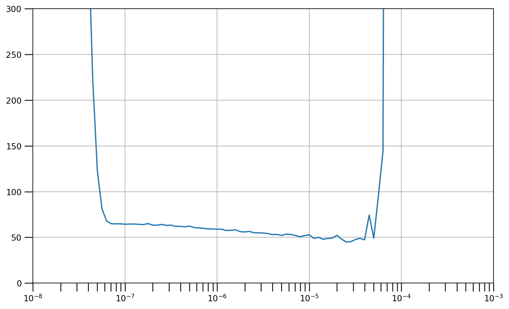

# Build the model
model_tune = tf.keras.models.Sequential([
  tf.keras.layers.Dense(10, activation="relu", input_shape=[window_size]),
  tf.keras.layers.Dense(10, activation="relu"),
  tf.keras.layers.Dense(1)
])

# Set the optimizer with the tuned learning rate
optimizer = tf.keras.optimizers.SGD(learning_rate=4e-6, momentum=0.9)

# Set the training parameters
model_tune.compile(loss="mse", optimizer=optimizer)

# Train the model
history = model_tune.fit(dataset, epochs=300,verbose=0)

# Plot all
loss = history.history['loss']
epochs = range(len(loss))
plot_loss = loss
plt.plot(epochs, plot_loss, 'b', label='Training Loss')
plt.show()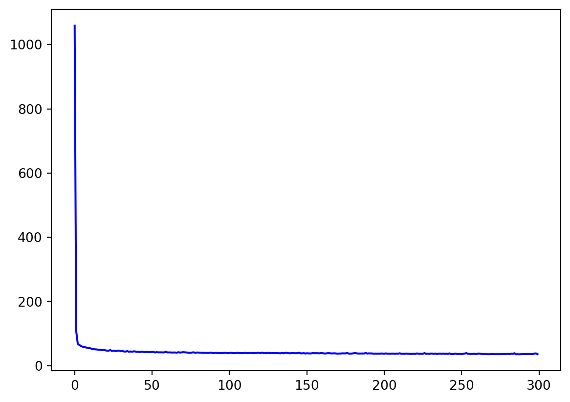

# Plot all excluding first 10
loss = history.history['loss']
epochs = range(10, len(loss))
plot_loss = loss[10:]
plt.plot(epochs, plot_loss, 'b', label='Training Loss')
plt.show()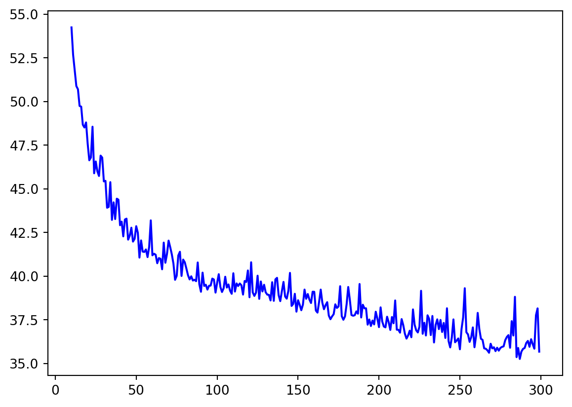

# Initialize a list
forecast = []

# Reduce the original series
forecast_series = series[split_time - window_size:]

# Use the model to predict data points per window size
for time in range(len(forecast_series) - window_size):
  forecast.append(model_tune.predict(forecast_series[time:time + window_size][np.newaxis]))

# Convert to a numpy array and drop single dimensional axes
results = np.array(forecast).squeeze()

# Plot the results
plot_series(time_valid, (x_valid, results))

print(tf.keras.metrics.mean_squared_error(x_valid, results).numpy())

42.02161

print(tf.keras.metrics.mean_absolute_error(x_valid, results).numpy())

4.852905

25 resource:

https://www.coursera.org/learn/tensorflow-sequences-time-series-and-prediction

https://github.com/https-deeplearning-ai/tensorflow-1-public/tree/main/C4