W4:Real-world time series data sunspots

Week 4 sunspots data

import tensorflow as tf
import numpy as np
import matplotlib.pyplot as plt

1 download data

import urllib.request

url="https://storage.googleapis.com/tensorflow-1-public/course4/Sunspots.csv"

urllib.request.urlretrieve(url, "Sunspots.csv")

('Sunspots.csv', <http.client.HTTPMessage at 0x291fef150>)

def plot_series(x, y, format="-", start=0, end=None, 
                title=None, xlabel=None, ylabel=None, legend=None ):
    """
    Visualizes time series data

    Args:
      x (array of int) - contains values for the x-axis
      y (array of int or tuple of arrays) - contains the values for the y-axis
      format (string) - line style when plotting the graph
      label (string) - tag for the line
      start (int) - first time step to plot
      end (int) - last time step to plot
      title (string) - title of the plot
      xlabel (string) - label for the x-axis
      ylabel (string) - label for the y-axis
      legend (list of strings) - legend for the plot
    """

    # Setup dimensions of the graph figure
    plt.figure(figsize=(10, 6))
    
    # Check if there are more than two series to plot
    if type(y) is tuple:

      # Loop over the y elements
      for y_curr in y:

        # Plot the x and current y values
        plt.plot(x[start:end], y_curr[start:end], format)

    else:
      # Plot the x and y values
      plt.plot(x[start:end], y[start:end], format)

    # Label the x-axis
    plt.xlabel(xlabel)

    # Label the y-axis
    plt.ylabel(ylabel)

    # Set the legend
    if legend:
      plt.legend(legend)

    # Set the title
    plt.title(title)

    # Overlay a grid on the graph
    plt.grid(True)

    # Draw the graph on screen
    plt.show()

2 read in data

import pandas as pd
data=pd.read_csv('./Sunspots.csv')
data.head()

	Unnamed: 0	Date	Monthly Mean Total Sunspot Number
0	0	1749-01-31	96.7
1	1	1749-02-28	104.3
2	2	1749-03-31	116.7
3	3	1749-04-30	92.8
4	4	1749-05-31	141.7

list(data)

['Unnamed: 0', 'Date', 'Monthly Mean Total Sunspot Number']

time=data['Unnamed: 0'].to_numpy()

series=data["Monthly Mean Total Sunspot Number"].to_numpy()

3 plot data

# Preview the data
plot_series(time, series, xlabel='Month', ylabel='Monthly Mean Total Sunspot Number')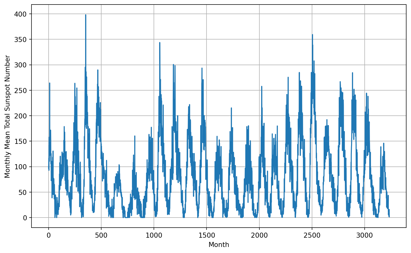

4 Split the Dataset

# Define the split time
split_time = 3000

# Get the train set 
time_train = time[:split_time]
x_train = series[:split_time]

# Get the validation set
time_valid = time[split_time:]
x_valid = series[split_time:]

5 Prepare Features and Labels

def windowed_dataset(series, window_size, batch_size, shuffle_buffer):
    """Generates dataset windows

    Args:
      series (array of float) - contains the values of the time series
      window_size (int) - the number of time steps to include in the feature
      batch_size (int) - the batch size
      shuffle_buffer(int) - buffer size to use for the shuffle method

    Returns:
      dataset (TF Dataset) - TF Dataset containing time windows
    """
  
    # Generate a TF Dataset from the series values
    dataset = tf.data.Dataset.from_tensor_slices(series)
    
    # Window the data but only take those with the specified size
    dataset = dataset.window(window_size + 1, shift=1, drop_remainder=True)
    
    # Flatten the windows by putting its elements in a single batch
    dataset = dataset.flat_map(lambda window: window.batch(window_size + 1))

    # Create tuples with features and labels 
    dataset = dataset.map(lambda window: (window[:-1], window[-1]))

    # Shuffle the windows
    dataset = dataset.shuffle(shuffle_buffer)
    
    # Create batches of windows
    dataset = dataset.batch(batch_size).prefetch(1)
    
    return dataset

# Parameters
window_size = 30
batch_size = 32
shuffle_buffer_size = 1000

# Generate the dataset windows
train_set = windowed_dataset(x_train, window_size, batch_size, shuffle_buffer_size)

6 DNN model

6.1 define DNN Model

# Reset states generated by Keras
tf.keras.backend.clear_session()


# Build the model
model = tf.keras.models.Sequential([
    tf.keras.layers.Dense(30, input_shape=[window_size], activation="relu"), 
    tf.keras.layers.Dense(10, activation="relu"),
    tf.keras.layers.Dense(1)
])

# Print the model summary
model.summary()

Model: "sequential"

┏━━━━━━━━━━━━━━━━━━━━━━━━━━━━━━━━━┳━━━━━━━━━━━━━━━━━━━━━━━━┳━━━━━━━━━━━━━━━┓
┃ Layer (type)                    ┃ Output Shape           ┃       Param # ┃
┡━━━━━━━━━━━━━━━━━━━━━━━━━━━━━━━━━╇━━━━━━━━━━━━━━━━━━━━━━━━╇━━━━━━━━━━━━━━━┩
│ dense (Dense)                   │ (None, 30)             │           930 │
├─────────────────────────────────┼────────────────────────┼───────────────┤
│ dense_1 (Dense)                 │ (None, 10)             │           310 │
├─────────────────────────────────┼────────────────────────┼───────────────┤
│ dense_2 (Dense)                 │ (None, 1)              │            11 │
└─────────────────────────────────┴────────────────────────┴───────────────┘

 Total params: 1,251 (4.89 KB)

 Trainable params: 1,251 (4.89 KB)

 Non-trainable params: 0 (0.00 B)

6.2 Tune the Learning Rate

# Set the learning rate scheduler
lr_schedule = tf.keras.callbacks.LearningRateScheduler(
    lambda epoch: 1e-8 * 10**(epoch / 20))

# Initialize the optimizer
optimizer = tf.keras.optimizers.SGD(momentum=0.9)

# Set the training parameters
model.compile(loss=tf.keras.losses.Huber(), optimizer=optimizer)

# Train the model
history = model.fit(train_set, epochs=100, callbacks=[lr_schedule],verbose=0)

# Define the learning rate array
lrs = 1e-8 * (10 ** (np.arange(100) / 20))

# Set the figure size
plt.figure(figsize=(10, 6))

# Set the grid
plt.grid(True)

# Plot the loss in log scale
plt.semilogx(lrs, history.history["loss"])

# Increase the tickmarks size
plt.tick_params('both', length=10, width=1, which='both')

# Set the plot boundaries
plt.axis([1e-8, 1e-3, 0, 100])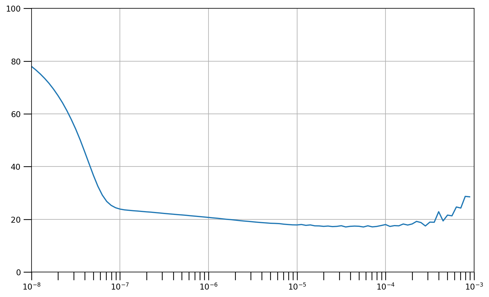

6.3 define DNN Model after tunned

# Reset states generated by Keras
tf.keras.backend.clear_session()

# Build the Model
model = tf.keras.models.Sequential([
    tf.keras.layers.Dense(30, input_shape=[window_size], activation="relu"), 
    tf.keras.layers.Dense(10, activation="relu"),
    tf.keras.layers.Dense(1)
])

6.4 complie model

# Set the learning rate
learning_rate = 2e-5

# Set the optimizer 
optimizer = tf.keras.optimizers.SGD(learning_rate=learning_rate, momentum=0.9)

# Set the training parameters
model.compile(loss=tf.keras.losses.Huber(),
              optimizer=optimizer,
              metrics=["mae"])

6.5 train DNN Model after tunned

# Train the model
history = model.fit(train_set,epochs=100,verbose=0)

6.6 Model Prediction

def model_forecast(model, series, window_size, batch_size):
    """Uses an input model to generate predictions on data windows

    Args:
      model (TF Keras Model) - model that accepts data windows
      series (array of float) - contains the values of the time series
      window_size (int) - the number of time steps to include in the window
      batch_size (int) - the batch size

    Returns:
      forecast (numpy array) - array containing predictions
    """

    # Generate a TF Dataset from the series values
    dataset = tf.data.Dataset.from_tensor_slices(series)

    # Window the data but only take those with the specified size
    dataset = dataset.window(window_size, shift=1, drop_remainder=True)

    # Flatten the windows by putting its elements in a single batch
    dataset = dataset.flat_map(lambda w: w.batch(window_size))
    
    # Create batches of windows
    dataset = dataset.batch(batch_size).prefetch(1)
    
    # Get predictions on the entire dataset
    forecast = model.predict(dataset)
    
    return forecast

forcast one value

forecast_series = series[split_time:split_time+window_size]
forecast = model_forecast(model, forecast_series, window_size, batch_size)

      1/Unknown 0s 18ms/step1/1 ━━━━━━━━━━━━━━━━━━━━ 0s 19ms/step

results = forecast.squeeze()
results

array(176.29543, dtype=float32)

# Reduce the original series
forecast_series = series[split_time-window_size:-1]

# Use helper function to generate predictions
forecast = model_forecast(model, forecast_series, window_size, batch_size)

# Drop single dimensional axis
results = forecast.squeeze()

# Plot the results
plot_series(time_valid, (x_valid, results))

WARNING:tensorflow:5 out of the last 18 calls to <function TensorFlowTrainer.make_predict_function.<locals>.one_step_on_data_distributed at 0x2a1cdb060> triggered tf.function retracing. Tracing is expensive and the excessive number of tracings could be due to (1) creating @tf.function repeatedly in a loop, (2) passing tensors with different shapes, (3) passing Python objects instead of tensors. For (1), please define your @tf.function outside of the loop. For (2), @tf.function has reduce_retracing=True option that can avoid unnecessary retracing. For (3), please refer to https://www.tensorflow.org/guide/function#controlling_retracing and https://www.tensorflow.org/api_docs/python/tf/function for  more details.
      1/Unknown 0s 19ms/step8/8 ━━━━━━━━━━━━━━━━━━━━ 0s 1ms/step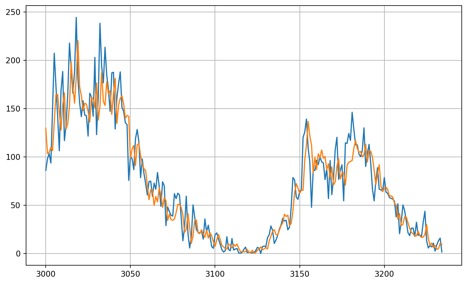

6.7 model result

## Compute the MAE and MSE
print(tf.keras.metrics.mean_squared_error(x_valid, results).numpy())

464.83243

print(tf.keras.metrics.mean_absolute_error(x_valid, results).numpy())

15.030133

7 RNN model

7.1 define RNN Model

# Build the Model
model = tf.keras.models.Sequential([
  tf.keras.layers.Conv1D(filters=64, kernel_size=3,
                      strides=1,
                      activation="relu",
                      padding='causal',
                      input_shape=[window_size, 1]),
  tf.keras.layers.LSTM(64, return_sequences=True),
  tf.keras.layers.LSTM(64),
  tf.keras.layers.Dense(30, activation="relu"),
  tf.keras.layers.Dense(10, activation="relu"),
  tf.keras.layers.Dense(1),
  tf.keras.layers.Lambda(lambda x: x * 400)
])

 # Print the model summary 
model.summary()

Model: "sequential_1"

┏━━━━━━━━━━━━━━━━━━━━━━━━━━━━━━━━━┳━━━━━━━━━━━━━━━━━━━━━━━━┳━━━━━━━━━━━━━━━┓
┃ Layer (type)                    ┃ Output Shape           ┃       Param # ┃
┡━━━━━━━━━━━━━━━━━━━━━━━━━━━━━━━━━╇━━━━━━━━━━━━━━━━━━━━━━━━╇━━━━━━━━━━━━━━━┩
│ conv1d (Conv1D)                 │ (None, 30, 64)         │           256 │
├─────────────────────────────────┼────────────────────────┼───────────────┤
│ lstm (LSTM)                     │ (None, 30, 64)         │        33,024 │
├─────────────────────────────────┼────────────────────────┼───────────────┤
│ lstm_1 (LSTM)                   │ (None, 64)             │        33,024 │
├─────────────────────────────────┼────────────────────────┼───────────────┤
│ dense_3 (Dense)                 │ (None, 30)             │         1,950 │
├─────────────────────────────────┼────────────────────────┼───────────────┤
│ dense_4 (Dense)                 │ (None, 10)             │           310 │
├─────────────────────────────────┼────────────────────────┼───────────────┤
│ dense_5 (Dense)                 │ (None, 1)              │            11 │
├─────────────────────────────────┼────────────────────────┼───────────────┤
│ lambda (Lambda)                 │ (None, 1)              │             0 │
└─────────────────────────────────┴────────────────────────┴───────────────┘

 Total params: 68,575 (267.87 KB)

 Trainable params: 68,575 (267.87 KB)

 Non-trainable params: 0 (0.00 B)

7.2 Tune the Learning Rate

# Get initial weights
init_weights = model.get_weights()

# Set the learning rate scheduler
lr_schedule = tf.keras.callbacks.LearningRateScheduler(
    lambda epoch: 1e-8 * 10**(epoch / 20))

# Initialize the optimizer
optimizer = tf.keras.optimizers.SGD(momentum=0.9)

# Set the training parameters
model.compile(loss=tf.keras.losses.Huber(), optimizer=optimizer)

# Train the model
history = model.fit(train_set, epochs=100, callbacks=[lr_schedule],verbose=0)

# Define the learning rate array
lrs = 1e-8 * (10 ** (np.arange(100) / 20))

# Set the figure size
plt.figure(figsize=(10, 6))

# Set the grid
plt.grid(True)

# Plot the loss in log scale
plt.semilogx(lrs, history.history["loss"])

# Increase the tickmarks size
plt.tick_params('both', length=10, width=1, which='both')

# Set the plot boundaries
plt.axis([1e-8, 1e-3, 0, 100])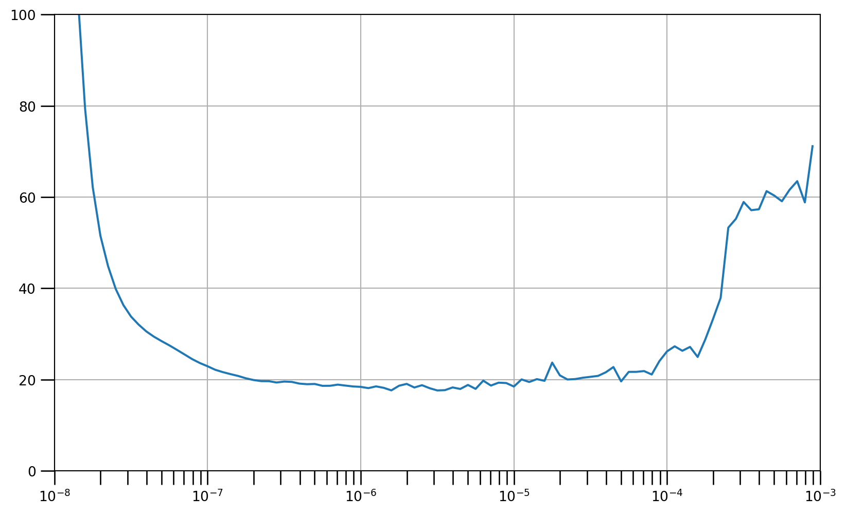

7.3 define RNN model after tunned

# Reset states generated by Keras
tf.keras.backend.clear_session()

# Reset the weights
model.set_weights(init_weights)

model.summary()

Model: "sequential_1"

┏━━━━━━━━━━━━━━━━━━━━━━━━━━━━━━━━━┳━━━━━━━━━━━━━━━━━━━━━━━━┳━━━━━━━━━━━━━━━┓
┃ Layer (type)                    ┃ Output Shape           ┃       Param # ┃
┡━━━━━━━━━━━━━━━━━━━━━━━━━━━━━━━━━╇━━━━━━━━━━━━━━━━━━━━━━━━╇━━━━━━━━━━━━━━━┩
│ conv1d (Conv1D)                 │ (None, 30, 64)         │           256 │
├─────────────────────────────────┼────────────────────────┼───────────────┤
│ lstm (LSTM)                     │ (None, 30, 64)         │        33,024 │
├─────────────────────────────────┼────────────────────────┼───────────────┤
│ lstm_1 (LSTM)                   │ (None, 64)             │        33,024 │
├─────────────────────────────────┼────────────────────────┼───────────────┤
│ dense_3 (Dense)                 │ (None, 30)             │         1,950 │
├─────────────────────────────────┼────────────────────────┼───────────────┤
│ dense_4 (Dense)                 │ (None, 10)             │           310 │
├─────────────────────────────────┼────────────────────────┼───────────────┤
│ dense_5 (Dense)                 │ (None, 1)              │            11 │
├─────────────────────────────────┼────────────────────────┼───────────────┤
│ lambda (Lambda)                 │ (None, 1)              │             0 │
└─────────────────────────────────┴────────────────────────┴───────────────┘

 Total params: 137,152 (535.75 KB)

 Trainable params: 68,575 (267.87 KB)

 Non-trainable params: 0 (0.00 B)

 Optimizer params: 68,577 (267.88 KB)

7.4 complie model

# Set the learning rate
learning_rate = 8e-7

# Set the optimizer 
optimizer = tf.keras.optimizers.SGD(learning_rate=learning_rate, momentum=0.9)

# Set the training parameters
model.compile(loss=tf.keras.losses.Huber(),
              optimizer=optimizer,
              metrics=["mae"])

7.5 train RNN Model after tunned

# Train the model
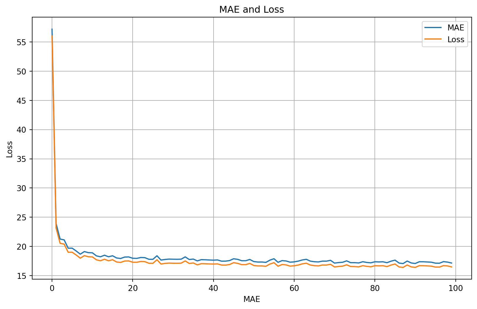
history = model.fit(train_set,epochs=100,verbose=0)

# Get mae and loss from history log
mae=history.history['mae']
loss=history.history['loss']

# Get number of epochs
epochs=range(len(loss)) 

# Plot mae and loss
plot_series(
    x=epochs, 
    y=(mae, loss), 
    title='MAE and Loss', 
    xlabel='MAE',
    ylabel='Loss',
    legend=['MAE', 'Loss']
    )

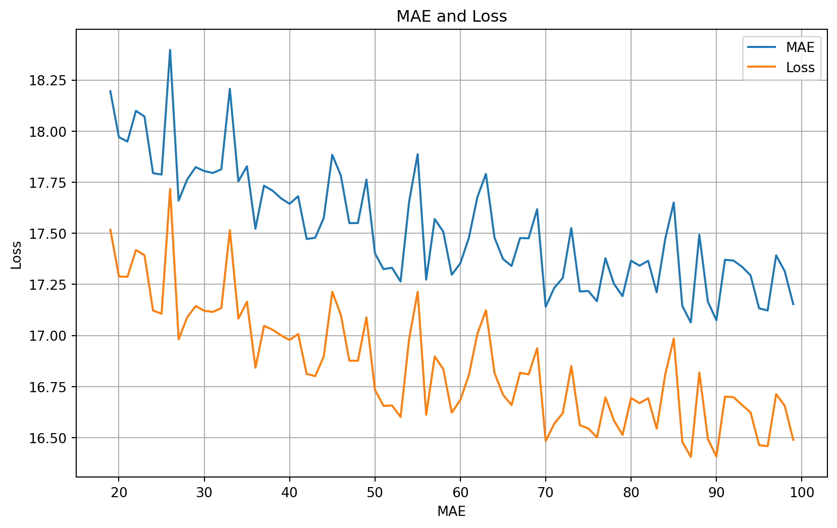
# Only plot the last 80% of the epochs
zoom_split = int(epochs[-1] * 0.2)
epochs_zoom = epochs[zoom_split:]
mae_zoom = mae[zoom_split:]
loss_zoom = loss[zoom_split:]

# Plot zoomed mae and loss
plot_series(
    x=epochs_zoom, 
    y=(mae_zoom, loss_zoom), 
    title='MAE and Loss', 
    xlabel='MAE',
    ylabel='Loss',
    legend=['MAE', 'Loss']
    )

7.6 Model Prediction

# Reduce the original series
forecast_series = series[split_time-window_size:-1]

# Use helper function to generate predictions
forecast = model_forecast(model, forecast_series, window_size, batch_size)

# Drop single dimensional axis
results = forecast.squeeze()

# Plot the results
plot_series(time_valid, (x_valid, results))

      1/Unknown 0s 153ms/step      8/Unknown 0s 23ms/step 8/8 ━━━━━━━━━━━━━━━━━━━━ 0s 24ms/step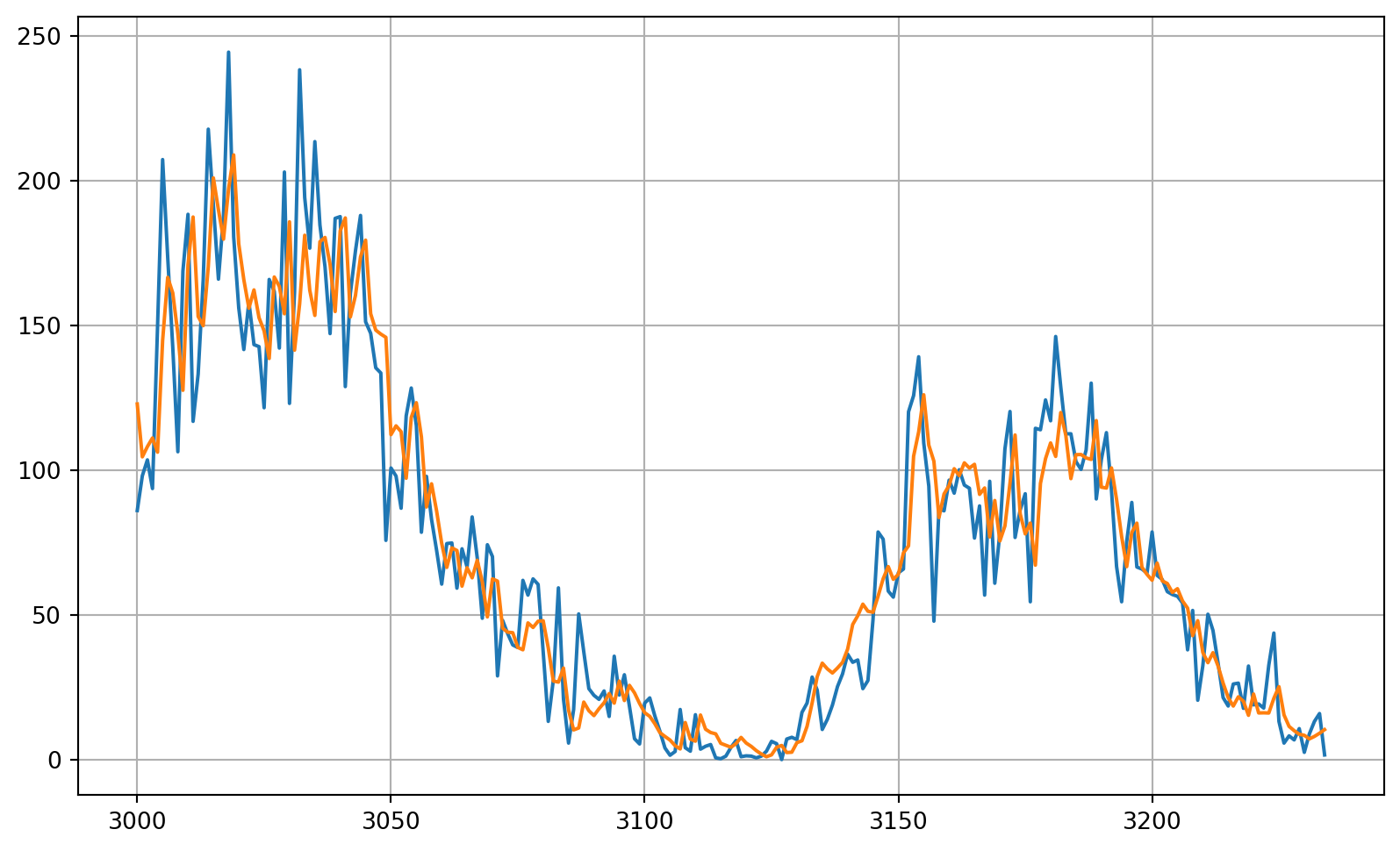

7.7 model result

## Compute the MAE and MSE
print(tf.keras.metrics.mean_squared_error(x_valid, results).numpy())

419.6377

print(tf.keras.metrics.mean_absolute_error(x_valid, results).numpy())

14.465482

8 resource:

https://www.coursera.org/learn/tensorflow-sequences-time-series-and-prediction

https://github.com/https-deeplearning-ai/tensorflow-1-public/tree/main/C4